Introduction
Overview
Teaching: 30 min
Exercises: 10 minQuestions
What is a command shell and why would I use one?
Objectives
Explain how the shell relates to the keyboard, the screen, the operating system, and users’ programs.
Explain when and why command-line interfaces should be used instead of graphical interfaces.
Open your terminal
To start we will open a terminal.
- Go to the link given to you at the workshop
- Paste the notebook link next to your name into your browser
- Select “Terminal” from the “JupyterLab” launcher (or blue button with a plus in the upper left corner)
- After you have done this put up a green sticky not if you see a flashing box next to a
$
What am I seeing: when the shell is first opened, you are presented with a prompt, indicating that the shell is waiting for input.
$
The Shell
The shell is a program where users can type commands. With the shell, it’s possible to invoke complicated programs like climate modeling software or simple commands that create an empty directory with only one line of code. The most popular Unix shell is Bash (the Bourne Again SHell — so-called because it’s derived from a shell written by Stephen Bourne). Bash is the default shell on most modern implementations of Unix and in most packages that provide Unix-like tools for Windows. Note that ‘Git Bash’ is a piece of software that enables Windows users to use a Bash like interface when interacting with Git.
Using the shell will take some effort and some time to learn. While a GUI presents you with choices to select, CLI choices are not automatically presented to you, so you must learn a few commands like new vocabulary in a language you’re studying. However, unlike a spoken language, a small number of “words” (i.e. commands) gets you a long way, and we’ll cover those essential few today.
The grammar of a shell allows you to combine existing tools into powerful pipelines and handle large volumes of data automatically. Sequences of commands can be written into a script, improving the reproducibility of workflows.
In addition, the command line is often the easiest way to interact with remote machines and supercomputers. Familiarity with the shell is near essential to run a variety of specialized tools and resources including high-performance computing systems. As clusters and cloud computing systems become more popular for scientific data crunching, being able to interact with the shell is becoming a necessary skill. We can build on the command-line skills covered here to tackle a wide range of scientific questions and computational challenges.
The Prompt
The shell typically uses $ as the prompt, but may use a different symbol.
In the examples for this lesson, we’ll show the prompt as $.
Most importantly, do not type the prompt when typing commands.
Only type the command that follows the prompt.
This rule applies both in these lessons and in lessons from other sources.
Also note that after you type a command, you have to press the Enter key to execute it.
The prompt is followed by a text cursor, a character that indicates the position where your typing will appear. The cursor is usually a flashing or solid block, but it can also be an underscore or a pipe. You may have seen it in a text editor program, for example.
Note that your prompt might look a little different. In particular, most popular shell
environments by default put your user name and the host name before the $. Such
a prompt might look like, e.g.:
student@workshop-1:~$
Read Evaluate Print Loop
There are many ways for a user to interact with a computer. For example, we often use a Graphical User Interface (GUI). With a GUI we might roll a mouse to the logo of a folder and click or tap (on a touch screen) to show the content of that folder. In a Commandline Interface the user can do all of the same actions (e.g. show the content of a folder). On the Commandline the user passes commands to the computer as lines of text. Below are the steps in a Read Evaluate Print Loop (REPL):
- the shell presents a prompt (like
$) - user types a command and presses the Enter key
- the computer reads it
- the computer executes it and prints its output (if any)
- loop from step #4 back to step #1
Reasons to learn about the shell
- Many bioinformatics tools can only process large data in the command line version not the GUI.
- The shell makes your work less boring (same set of tasks with a large number of files)
- The shell makes your work less error-prone
- The shell makes your work more reproducible.
- Many bioinformatic tasks require large amounts of computing power
Let’s call some programs
The most basic command is to call a program to perform its default action. For example, call the program
whoamito return your username.whoamiYou can also call a program and pass arguments to the program, for example this command to find which shell we are using:
echo $SHELL
Glance at the Filesystem
The ls command will list the contents of
your current directory (directory is synonymous with folder). Any line that starts with # will not be executed. We can write comments to ourselves by starting the line with #.
# call ls to list current directory
ls

# pass one or more paths of files or directories as argument(s)
ls /home/student/
In a GUI you may customize your finder/file browser based on how you like to search. In general if you can do it on a GUI there is a way to use text to do it on the commandline. I like to see my most recently changed files first. I also like to see the date they were edited.
# call ls to list bin and show the most recently changed files first (with the `-t` option/flag)
ls -t /home/student/

# add the `-l` to show who owns the file, file size, and what date is was last edited
ls -t -l /home/student/

# a flags to distinguish Folders from files (`-F`) and to show "human readable" filesizes (`-h`)
ls -t -l -F -h /home/student/

# combine short flags for faster typing
ls -lthF /home/student/
The basic syntax of a unix command is:
- call the program
- pass any flags/options
- pass any “order dependent arguments”
Getting help
ls has lots of other options. There are common ways to find out how to use a command and what options it
accepts (depending on your environment). Today we will call the unix command man and pass the name of the program that we want a manual for as the argument for man.
$ man ls
Usage: ls [OPTION]... [FILE]...
List information about the FILEs (the current directory by default).
Sort entries alphabetically if none of -cftuvSUX nor --sort is specified.

Mandatory arguments to long options are mandatory for short options too.
  -a, --all                  do not ignore entries starting with .
  -A, --almost-all           do not list implied . and ..
      --author               with -l, print the author of each file
  -b, --escape               print C-style escapes for nongraphic characters
Help menus show you the basic syntax of the command. Optional elements are shown in square brackets. Ellipses indicate that you can type more than one of the elements.
Help menus show both the long and short version of the flags. Use the short option when typing commands directly into the shell to minimize keystrokes and get your task done faster. Use the long option in scripts to provide clarity. It will be read many times and typed once.
When
mandoes not workIf
man PROGRAMdoes not show you a help menu there are other common ways to show help menus that you can try.
- call the program with only the
--helpflag Typeqto exit out of this help screen.- some bioinformatics programs will show a help menu if you call the tool without any flags or arguments (e.g.
samtools).
Command not found
If the shell can’t find a program whose name is the command you typed, it will print an error message such as:
$ ksSolution
ks: command not foundThis might happen if the command was mis-typed or if the program corresponding to that command is not installed. When your get an error message stay calm and give it a couple of read throughs. Error messages can seem akwardly worded at first but they can really help guide your debugging.
The Cloud
There are a number of reasons why accessing a remote machine is invaluable to any scientists working with large datasets. In the early history of computing, working on a remote machine was standard practice - computers were bulky and expensive. Today we work on laptops or desktops that are more powerful than the sum of the world’s computing capacity 20 years ago, but many analyses (especially in genomics) are too large to run on these laptops/desktops. These analyses require larger machines, often several of them linked together, where remote access is the only practical solution.
Schools and research organizations often link many computers into one High Performance Computing (HPC) cluster on or near the campus. Another model that is becoming common is to “rent” space on a cluster(s) owned by a large company (Amazon, Google, Microsoft, etc). In recent years, computational power has become a commodity and entire companies have been built around a business model that allows you to “rent” one or more linked computers for as long as you require, at lower cost than owning the cluster (depending on how often it is used vs idle, etc). This is the basic principle behind the cloud. You define your computational requirements and off you go.
The cloud is a part of our everyday life (e.g. using Amazon, Google, Netflix, or an ATM involves remote computing). The topic is fascinating, but this lesson says a few minutes or less so let’s get back to working on it for the workshop.
For this workshop starting a vm and setting up your working environment has been done for you. Going forward reach out to your organizations system administrators for your cluster for suggestions. To read more on your own here are lessons about working on the cloud and a local HPC. Additional lesson’s that you can run from a remote computer:
HUMAN GENOMIC DATA & SECURITY
Note that if you are working with human genomics data there might be ethical and legal considerations that affect your choice of cloud resources to use. The terms of use, and/or the legislation under which you are handling the genomic data, might impose heightened information security measures for the computing environment in which you intend to process it. This is a too broad topic to discuss in detail here, but in general terms you should think through the technical and procedural measures needed to ensure that the confidentiality and integrity of the human data you work with is not breached. If there are laws that govern these issues in the jurisdiction in which you work, be sure that the cloud service provider you use can certify that they support the necessary measures. Also note that there might exist restrictions for use of cloud service providers that operate in other jurisdictions than your own, either by how the data was consented by the research subjects or by the jurisdiction under which you operate. Do consult the legal office of your institution for guidance when processing human genomic data.
Key Points
Many bioinformatics tools can only process large data in the command line version not the GUI.
The shell makes your work less boring (same set of tasks with a large number of files)”
The shell makes your work less error-prone
The shell makes your work more reproducible.
Many bioinformatic tasks require large amounts of computing power
Navigating and Editing Files
Overview
Teaching: 4h min
Exercises: 30m minQuestions
How can I move around on the computer/vm?
How can I see what files and directories I have?
How can I specify the location of a file or directory on the computer/vm?
How can I specify the location of a file or directory in a bucket?
Objectives
Translate an absolute path into a relative path and vice versa.
Construct absolute and relative paths that identify specific files and directories.
Use options and arguments to change the behaviour of a shell command.
Demonstrate the use of tab completion and explain its advantages.
The Filesystem
The part of the operating system responsible for managing files and directories is called the file system. It organizes our data into files, which hold information, and directories (also called ‘folders’), which hold files or other directories.
Several commands are frequently used to create, inspect, rename, and delete files and directories. To start exploring them, we’ll go to our open shell window.
First, let’s find out where we are by running a command called pwd (which stands for ‘print working directory’). Directories are like places — at any time while we are using the shell, we are in exactly one place called our current working directory. Commands mostly read and write files in the current working directory, i.e. ‘here’, so knowing where you are before running a command is important. pwd shows you where you are:
$ pwd
Here, the response may be different on different computers. Often a session begins in the users home directory.
To understand what a file system is, let’s have a look at how the file system as a whole is organized. For the sake of this example, we’ll be illustrating a portion of the file system on our workshop VM. After this illustration, you’ll be learning commands to explore your own filesystem, which will be constructed in a similar way, but not be exactly identical.
On the workshop VM, part of the filesystem looks like this:
$ tree -L 2 /data/RNA/
/data/RNA/
├── bulk
│   ├── airway_raw_counts.csv.gz
│   └── airway_sample_metadata.csv
└── single_cell
    └── README
Another way to diagram the filesystem is like this. The root directory is always named /.

Relative Paths
/ : root directory
Absolute Path : a path that starts from the root of the file system. Any path that starts with / is an absolute path.
Relative Path : a path that starts from current location or any location other than the root.
. : current working directory
cd /data/alignment/references/
ls ./GRCh38_1000genomes/
.. : one level up directory, also known as the parent directory of the current directory
ls -F ../
ls -F ../combined
ls -a
~ : user’s home directory
ls -F ~/
cd : a command to change your current working directory
- : previous directory. The dash is interpreted as the last directory that the user was in.
cd -
Note: if no special characters are used UNIX assumes your path begins in the current working directory
Create a Relative Path
Without changing directories create a relative path to list the contents of the
/data/alignment/combineddirectory (showing a trailing slash to see which are directories). For the second part of the code challenge, what does the commandcdwithout a directory name do?$ cd /data/alignment/references/GRCh38_1000genomes/Solution
ls -F ../../combined/Second part: changes the current working directory to the home directory
Software on the File System the PATH Variable
Commands like ls and (on our VM) samtools seem to exist as special words that the user can type to call a single version of a program. However, these programs are actual files on the file system that we can call because they are in one of the many locations that the shell knows to search when a command is executed.
How can we run samtools when we don’t see any program named samtools in our current working directory?
Location of Samtools
# generate a samtools help menu
samtools
# show the absolute path to samtools
which samtools
VM path for samtools
/home/student/miniconda3/envs/siw/bin/samtools
Location of ls
# show the absolute path to ls
which ls
VM path for ls
/usr/bin/ls
you or a systems administrator will probably install some bioinformatics programs that researchers use commonly
In this workshop those have been installed at /home/student/miniconda3/envs/siw/bin using a environment manager called
conda. Ask your systems administrators to assist with software installation and/or tips
for installing tools.
What if we want to know the version of samtools?
samtools --version
samtools 1.20
Using htslib 1.20
Copyright (C) 2024 Genome Research Ltd.

Samtools compilation details:
   Features:       build=configure curses=yes
   CC:             /opt/conda/conda-bld/samtools_1720645213030/_build_env/bin/x86_64-conda-linu
...
You may want to start with the most recent version of a tool or need to use a previous tool to match prior analysis runs. It can be useful to record the absolute path to bioinformatics tools in commands that you run for publication or intend to have to run again in a consistant fashion. It can also be useful to include the bioinformatics tool version in the path to the tool for clarity.
If you are just glancing at the alignment header to see what genome it was aligned to (e.g. GRCh38) then you don’t need to be so explicit.
$ samtools view -H /data/alignment/combined/NA12878.dedup.bam
...
@RG     ID:NA12878_TTGCCTAG-ACCACTTA_HCLHLDSXX_L001     PL:illumina     PM:Unknown      LB:NA12878      DS:GRCh38       SM:NA12878       CN:NYGenome     PU:HCLHLDSXX.1.TTGCCTAG
@RG     ID:NA12878_TTGCCTAG-ACCACTTA_HCLHLDSXX_L002     PL:illumina     PM:Unknown      LB:NA12878      DS:GRCh38       SM:NA12878       CN:NYGenome     PU:HCLHLDSXX.2.TTGCCTAG
@RG     ID:NA12878_TTGCCTAG-ACCACTTA_HCLHLDSXX_L003     PL:illumina     PM:Unknown      LB:NA12878      DS:GRCh38       SM:NA12878       CN:NYGenome     PU:HCLHLDSXX.3.TTGCCTAG
...
How the Shell Finds Programs
The PATH environment variables defines the shell’s search path.
In the shell a variable is defined without a starting dollar sign but when the value
of the variable is retrived you add the $ begining of the variable name. Tips: also wrap the variable name in curly braces {} so that the shell can clearly see the last character that belongs to the variable name. There cannot be a space on either side of the = sign.
# define a variable
$ project_name="LUAD"
# retrieve the value of the variable
echo ${LUAD}
# use export to define the variable for the shell session and for any programs called during the session
$ export project_name="LUAD"
When you run a command like ls or samtools, the shell splits $PATH into components to get a list of directories.
Unix uses : as a separator. The shell looks for the program in each directory in left-to-right.
Then the shell runs the first program with that name that it finds.
which reported that samtools was in /home/student/miniconda3/envs/siw/bin/. This is the second directory listed in our $PATH.
$ echo $PATH
/home/student/bin:/home/student/miniconda3/envs/siw/bin:/home/student/miniconda3/condabin:/usr/local/sbin:/usr/local/bin:/usr/sbin:/usr/bin:/snap/bin:/software/manta-1.6.0.centos6_x86_64/bin:/home/student/paragraph-v2.4a/bin:/home/student/gatk-4.6.0.0
You can add a path for a tool that you need to your path. Make sure to also redefine the current $PATH variable as the last portion of the path. Otherwise you may lose the ability to run cd, ls, etc.
$ export PATH=/NEW_PATH/:$PATH
CLI typing hints
- Tab : autocompletes paths (use this for speed and to avoid mistakes !!)
- ↑/↓ arrow : moves through previous commands
- Ctrla : goes to the beginning of a line
- Ctrle: goes to the end of the line
- short flags generally
-followed by a single letter- long flags generally
--followed by a word- flags are often called options in manuals (both terms are correct)
- command/program will be used interchangeably (a whole line of code is also called a command)
- To list your past commands: Type
historyin the command line
Buckets (not covered in workshop)
On your computer files are often stored “locally” on that computer in a directory. On the cloud permanent storage areas are called a “bucket.” The console that we are using is running on an ephemeral virtual machine (VM). We will copy files to our vm or read them from the bucket to use them. Any file we create or modify in our vm will be deleted when we turn off the vm. If your lab is working on the cloud then users will use a bucket to save files needed for analysis after the vm is stopped.
On google cloud the program gcloud storage allows you to run ls and cp commands to search and transfer files between VMs and your buckets.
Example of a file in a bucket
List a file in a bucket:
gcloud storage ls gs://genomics-public-data/resources/broad/hg38/v0/wgs_calling_regions.hg38.interval_listCopy a file from a bucket to your current working directory.
gcloud storage cp gs://genomics-public-data/resources/broad/hg38/v0/wgs_calling_regions.hg38.interval_list .
Key Points
The file system is responsible for managing information on the disk.
Information is stored in files, which are stored in directories (folders).
Directories can also store other directories, which then form a directory tree.
The command
pwdprints the user’s current working directory.The command
ls [path]prints a listing of a specific file or directory;lson its own lists the current working directory.The command
cd [path]changes the current working directory.Most commands take options that begin with a single
-.Directory names in a path are separated with
/on Unix.Slash (
/) on its own is the root directory of the whole file system.An absolute path specifies a location from the root of the file system.
A relative path specifies a location starting from any location other than the root.
A
~indicates your home directoryA
-indicates the last directory that you were inDot (
.) on its own means ‘the current directory’;..means ‘the directory above the current one’.
Working With Files and Directories
Overview
Teaching: 31h min
Exercises: 20 minQuestions
How can I create, copy, and delete files and directories?
How can I edit files?
Objectives
Delete, copy and move specified files and/or directories.
Create files in that hierarchy using an editor or by copying and renaming existing files.
Creating directories
We now know how to explore files and directories, but how do we create them in the first place?
In this episode we will learn about creating and moving files and directories, using our home directory.
First we see where we are and what we already have. We want to be in the home directory on the Desktop, which we can check using:
pwd
# if needed we can change to the home directory with
cd
Let’s create a new directory called workshop using the command mkdir (which has no output)
mkdir : make directory
mkdir workshop
ls -F ~/
mkdir workshop/output/
mkdir workshop/logs/
mkdir workshop/scripts/
mkdir workshop/mock_data/
mkdir workshop/mock_data/fasta/
touch : create new, empty files
touch genome.fa
vi : a plain text editor that is already installed on many linux computers. This is not the most user-friendly plain text editor. A more user-friendly option is BBEdit. You may independtly install this on your laptop if you need an editor for future programming tasks. It is free and allows you edit custom scripts that are stored on a remote cluster.
vi genome.fa
In vi type i. Then type out a few FASTA records. Like the ones below.
When you are finished editing type esc, then type :wq follwed by return to save and quit.
>chr1
AACCGCGCGTACGCGCGCGCGC
CTCTACNNNNNN
>chr2
TGTGTCTGAAANTGTCATGTCA
NNNTCNTGTGTGTGAAAAAAAA
NNTGCNA
>chr3
AACCGCGCGTATCTGAACGCGC
CTCTAAATCGAT
cp : copy file(s) to a new location
# makes a copy with the same filename
cp ~/genomes.fa ~/workshop/mock_data/fasta/
# makes a copy with a new filename (both .fa and .fasta and .fna are valid FASTA file suffixes)
cp ~/genomes.fa ~/genomes.fasta
# see new file
ls -thl ~/genomes.fa ~/workshop/mock_data/fasta/
mv : move files or directories (if they are moved in the same location then they are renamed)
mv ~/genomes.fasta ~/workshop/mock_data/fasta/
mv ~/genomes.fa ~/new_name_genomes.fa
rm : remove file (CAUTION: no undelete here !!)
rm ~/new_name_genomes.fa
rmdir : remove empty directory
mkdir ~/workshop/mock_data/wrong
rmdir ~/workshop/mock_data/wrong
File permissions
chmod : command to set permissions of a file or directory
ls -thl ~/workshop/mock_data/fasta/genomes.fa
The command ls -thl lists the files in the current folder and displays them in the long listing format. While this may initially look complex, we can break this down in the following left to right order:
A set of ten permission flags
- Link count (which is irrelevant to this course)
- The owner of the file
- The associated group
- The size of the file
- The data that the file was last modified
- The name of the file
- The permission flags are the important thing we want to look at here. We can further break these down into the following three basic
Permission Types:
- Read - Which refers to a user’s capability to read the contents of the file.
- Write - Which refer to a user’s capability to write or modify a file or directory.
- Execute - Which affects a user’s capability to execute a file or view the contents of a directory.
Each of these permission types is listed in the _rwxrwxrwx section of the ls output. The first character marked by an underscore is the special permission flag that can vary. It shows things like whether the item is a directory.
The following set of three characters (rwx) is for the owner permissions.
The second set of three characters (rwx) is for the Group permissions.
The third set of three characters (rwx) is for the All Users permissions.
See all options at http://www.onlineconversion.com/html_chmod_calculator.html.
- The value
7is the file/directory can be read, written to and executed. - With a
5the file/directory can be read and executed (but not written to!). - With a
0the file/directory can’t be read, written to or executed.
Your bioinformatics sequence and reference files should be read only.
chmod -R 550 ~/workshop/mock_data/fasta
echo "oops" > ~/workshop/mock_data/fasta/genomes.fa
Tokens and key files work something like passwords and should be read only by you (with no permissions for your group and other users).
touch ~/workshop/logs/gdc_token_example.txt
chmod  500 ~/workshop/logs/gdc_token_example.txt
Key Points
Repeating yourself
Overview
Teaching: 30 min
Exercises: 20 minQuestions
How can I combine existing commands to produce a desired output?
How can I perform the same actions on many different files?
How can I save and re-use commands?
Objectives
Explain the advantage of linking commands with pipes and filters.
Redirect a command’s output to a file.
Write a loop that applies one or more commands separately to each file in a set of files.
Trace the values taken on by a loop variable during execution of the loop.
Explain the difference between a variable’s name and its value.
Write a shell script that runs a command or series of commands for a fixed set of files.
Run a shell script from the command line.
Pipes and Filters
Now that we know a few basic commands, we can finally look at the shell’s most powerful feature:
the ease with which it lets us combine existing programs in new ways.
We’ll start with the directory /data/alignment/references/GRCh38_1000genomes/ that contains GRCh38 reference files.
The .fa extension indicates that a files is in FASTA format, a simple text format that specifies the nucleic or amino acid sequences.
head : returns the first lines of a file (default number of lines is 10)
tail : returns the last lines of a file (default number of lines is 10)
$ cd /data/alignment/references/GRCh38_1000genomes/
$ head GRCh38_full_analysis_set_plus_decoy_hla.fa
$ tail GRCh38_full_analysis_set_plus_decoy_hla.fa
grep : program to find lines that match a pattern
^ : regex (regular expression) which matches the first character
| : pipes output from the command on the left as input to the command on the right
The vertical bar, |, between the two commands is called a pipe. It tells the shell that we want to use the output of the command on the left as the input to the command on the right. Nothing prevents us from chaining pipes consecutively. We can for example send the output of head directly to grep, and then send the resulting output to sort (a command that sorts lines of text). This removes the need for any intermediate files.
This idea of linking programs together is why Unix has been so successful. Instead of creating enormous programs that try to do many different things, Unix programmers focus on creating lots of simple tools that each do one job well, and that work well with each other. This programming model is called ‘pipes and filters’. We’ve already seen pipes; a filter is a program like wc or sort that transforms a stream of input into a stream of output. Almost all of the standard Unix tools can work this way. Unless told to do otherwise, they read from standard input, do something with what they’ve read, and write to standard output.
The key is that any program that reads lines of text from standard input and writes lines of text to standard output can be combined with every other program that behaves this way as well. You can and should write your programs this way so that you and other people can put those programs into pipes to multiply their power.
$ # returns lines that contain GRCh38
$ cat GRCh38_full_analysis_set_plus_decoy_hla.fa | grep "GRCh38"
$ # returns lines that start with (^) the > symbol
$ cat GRCh38_full_analysis_set_plus_decoy_hla.fa | grep "^>"
$ # counts lines that start with (^) the > symbol
$ cat GRCh38_full_analysis_set_plus_decoy_hla.fa | grep -c "^>"
* : glob (this translates to zero of more of any character)
$ ls /data/alignment/references/*/*fa
$ cat /data/alignment/references/*/*fa | grep -c "^>"
Writing to files
> : redirects output to a file
The greater than symbol, >, tells the shell to redirect the command’s output to a file instead of printing it to the screen. This command prints no screen output, because everything that wc would have printed has gone into the file lengths.txt instead. If the file doesn’t exist prior to issuing the command, the shell will create the file. If the file exists already, it will be silently overwritten, which may lead to data loss. Thus, redirect commands require caution.
$ cat /data/alignment/references/*/*fa | grep -c "^>" > ~/workshop/output/seq_counts.txt
$ cat ~/workshop/output/seq_counts.txt
>> : appends output to the end of a file
$ cat /data/alignment/references/*/*fa | grep -c "^>" >> ~/workshop/output/seq_counts.txt
$ cat ~/workshop/output/seq_counts.txt
Loops
Loops are a programming construct which allow us to repeat a command or set of commands for each item in a list. As such they are key to productivity improvements through automation. Similar to wildcards and tab completion, using loops also reduces the amount of typing required (and hence reduces the number of typing mistakes).
Suppose we have dozens of genome sequence alignment files in SAM, BAM or CRAM format. For this example, we’ll use the /data/*/*cram files which only have two example files, but the principles can be applied to many many more files at once.
The structure of these files is the same and that allows many tools (including QC tools to evaluate them). Let’s look at the files:
$ # the header describes the reference and read groups
$ samtools view -H /data/alignment/combined/NA12878.dedup.bam
$ # the first three alignments are printed to the screen to look at
$ samtools view /data/alignment/combined/NA12878.dedup.bam | head -3
We would like to get QC metrics for each alignment file. For each file, we would need to execute the command samtools flagstat. We’ll use a loop to solve this problem, but first let’s look at the general form of a loop, using the pseudo-code below:
# The word "for" indicates the start of a "For-loop" command
for thing in list_of_things
#The word "do" indicates the start of job execution list
do
    # Indentation within the loop is not required, but aids legibility
    operation_using/command $thing
# The word "done" indicates the end of a loop
done
and we can apply this to our example like this:
for cram in /data/*/*cram; do
    echo ${cram}
    echo "working..."
    samtools flagstat ${cram}
    echo "done"
done
Follow the Prompt
The shell prompt changes from
$to>and back again as we were typing in our loop. The second prompt,>, is different to remind us that we haven’t finished typing a complete command yet. A semicolon,;, can be used to separate two commands written on a single line.
When the shell sees the keyword for, it knows to repeat a command (or group of commands) once for each item in a list. Each time the loop runs (called an iteration), an item in the list is assigned in sequence to the variable, and the commands inside the loop are executed, before moving on to the next item in the list. Inside the loop, we call for the variable’s value by putting $ in front of it. The $ tells the shell interpreter to treat the variable as a variable name and substitute its value in its place, rather than treat it as text or an external command.
In this example, the list is three filenames: /data/cancer_genomics/COLO-829BL_1B.variantRegions.cram and /data/cancer_genomics/COLO-829_2B.variantRegions.cram. Each time the loop iterates, we first use echo to print the value that the variable ${cram} currently holds. This is not necessary for the result, but beneficial for us here to have an easier time to follow along. Next, we will run the flagstat command on the file currently referred to by ${cram}. The first time through the loop, ${cram} is COLO-829BL_1B.variantRegions.cram. The interpreter runs the command head on COLO-829BL_1B.variantRegions.cram and prints the QC metrics. For the second iteration, ${cram} becomes COLO-829_2B.variantRegions.cram. This time, the shell runs head on COLO-829_2B.variantRegions.cram and prints the QC metrics. Since the list was only two items, the shell exits the for loop.
Same Symbols, Different Meanings
Here we see
>being used as a shell prompt, whereas>is also used to redirect output. Similarly,$is used as a shell prompt, but, as we saw earlier, it is also used to ask the shell to get the value of a variable.If the shell prints
>or$then it expects you to type something, and the symbol is a prompt.If you type
>or$yourself, it is an instruction from you that the shell should redirect output or get the value of a variable.
When using variables it is good practice to put the names into curly braces to clearly delimit the variable name: $cram is equivalent to ${cram}, but is different from ${cr}am. You may find this notation in other people’s programs.
We have called the variable in this loop cram in order to make its purpose clearer to human readers. The shell itself doesn’t care what the variable is called; if we wrote this loop as:
for x in /data/*/*cram; do
    echo ${x}
    echo "working..."
    samtools flagstat ${x}
    echo "done"
done
It would work exactly the same way. Don’t do this. Programs are only useful if people can understand them, so meaningless names (like x) or misleading names (like temperature) increase the odds that the program won’t do what its readers think it does.
In the above examples, the variables (thing, filename, x and temperature) could have been given any other name, as long as it is meaningful to both the person writing the code and the person reading it.
Note also that loops can be used for other things than filenames, like a list of numbers or a subset of data.
Key Points
wc counts lines, words, and characters in its inputs (see SWC primer).
cat displays the contents of its inputs.
sort sorts its inputs (see SWC primer).
head displays the first 10 lines of its input by default without additional arguments.
tail displays the last 10 lines of its input by default without additional arguments.
command > [file] redirects a command’s output to a file (overwriting any existing content!!).
command >> [file] appends a command’s output to a file.
first | second is a pipeline. The output of the first command is used as the input to the second.
The best way to use the shell is to use pipes to combine simple single-purpose programs (filters)
A for loop repeats commands once for every thing in a list.
Every for loop needs a variable to refer to the thing it is currently operating on.
Use $name to expand a variable (i.e., get its value). ${name} can also be used.
Do not use spaces, quotes, or wildcard characters such as * or ? in filenames, as it complicates variable expansion.
Give files consistent names that are easy to match with wildcard patterns to make it easy to select them for looping.
Use the ↑/↓ keys to scroll through previous commands to edit and repeat them.
Use Ctrl+R to search through the previously entered commands (see SWC primer).
Use history to display recent commands, and !number to repeat a command by number (see SWC primer).
Save commands in files (usually called shell scripts) for re-use.
bash filename runs the commands saved in a file.
$@ refers to all of a shell script’s command-line arguments (see SWC primer).
$1, $2, etc., refer to the first command-line argument, the second command-line argument, etc.
Place variables in quotes if the values might have spaces in them.
Read Alignment and Small Variant Calling
Overview
Teaching: min
Exercises: minQuestions
Objectives
Intro to Alignment Lecture
https://drive.google.com/file/d/1HysQvr9pEj0DInCuF9oBqHCpzA2ZlUDT/view?usp=sharing
Getting Started
Log in to your instances through Jupyter notebooks and launch a terminal.
Next, find the places in the directories where you are going to work.
All of the data you will need for these exercises are in
/data/alignment
There are multiple subdirectories inside that directory that you will access for various parts of this session. Part of the aim of these exercises is for you to become more familiar with working with files and commands in addition to learning the processing steps, so for the most part there will not be full paths to the files you need, but all of them will be under the alignment directory.
You CAN put your output anywhere you want to. That’s also part of the workshop. I would recommend you use the following space:
/workshop/output
I would recommend making a directory under that for everything to keep it separate from what you did yesterday or will do in the following sessions. You could do something like
mkdir /workshop/output/alignment
However, if you think you will find it confusing to have “alignment” in both in the input and output directory paths, you could try something different like align_out or alnout or whatever you want. It’s only important that you remember it.
Part of this work will require accessing all the various data and feeding it into the programs you will run and directing your output. Certain steps will require that you be able to find the output of previous steps to use it for the input to the next steps. Keeping your work organized this way is a key part of running multi-step analysis pipelines. Yesterday we discussed absolute and relative paths. During this session you will need to keep track of where you are in the filesystem (pwd), how to access your input data from there, and how to access your output files and directories from there.
It is up to you if you want to do everything with absolute paths, with relative paths, or a mix. It is up to you if you want to cd to the output directory, the input directory, or a third place. Do whichever feels most comfortable to you. Note that if you choose to do everything with absolute paths, your working directory does not matter, but you will type more.
Tab completion is your friend. If there are only three things I want you to remember from this workshop, they are tab completion, tab completion, and tab completion.
Copy and Paste
Copy and paste is not your friend. It may be possible to copy and paste commands from this markdown into the Jupyter terminal. Please note that this more often than not fails in general because text in html or pdf or Word documents has non-printing characters or non-standard punctuation (like em dashes and directional quotation marks) which are not processed by the unix shell and will generate errors. The same is true with copying text that spans multiple lines. Because of this, most of the code blocks in this section are intentionally constructed to prevent copying and pasting. That is, the commands will be constructed, but full paths will not be given and real names of files will be substituted with placeholders. As a convention, if a name is in UPPERCASE ITALIC or as _UPPERCASE_, it is the placeholder for a filename or directory name you need to provide. If you copy and paste this, it will fail to work.
The exercises we will do
What we will do today is take some data from the Genome in a Bottle sample, also part of 1000 Genomes, NA12878, and this person’s parents, NA12891 and NA12892, and align them to the human genome. Aligning a whole human genome would take hours, and analyzing it even longer, so I have extracted a subset of reads that align to only chromosome 20, which is about 2% of the genome and will align in a reasonable amount of time. We will still align to the entire genome, because you should always align to the whole genome even if you think you have only targeted a piece of it because there are always off target reads, and using the whole genome for alignment improves alignment quality. We will walk through the following steps:
- Build an index for the bwa aligner (on a small part of the genome)
- Align reads to the genome with bwa mem
- Merge multiple alignment files and sort them in coordinate order (with gatk or samtools)
- Mark duplicate reads with gatk
- Call variants using gatk HaplotypeCaller (on a small section of chromosome 20)
- Filter variants using gatk VariantFiltration
We will also skip a couple of steps, indel realignment and base quality score recalibration (BQSR), but we will discuss them.
Along the way we will discuss the formatting and uses of several file formats:
- fasta
- fastq
- sam
- bam
- cram
- gatk dup metrics
- vcf
- gvcf
Running bwa
bwa is the Burrow-Wheeler Aligner. We’re going to use it to align short reads.
First we’re going to see an example of building the bwt index. Indexing an entire human genome would again take an hour or more, so we will just index chromosome 20. Look for it in the references subdirectory of /data/alignment and make a copy of it to your workspace using cp then index it with bwa. This should take about 1 minute.
cp /data/alignment/references/chr20.fa _MYCHR20COPY_
bwa index -a bwtsw _MYCHR20COPY_
The -a bwtsw tells bwa which indexing method to use. It also supports other indexing schemes that are faster for small genomes (up to a few megabases, like bacteria or most fungi) but do not scale to vertebrate sized genomes. You can see more detail about this by running bwa index with no other arguments, which produces the usage.
If you now look in the directory where you put MYCHR20COPY, you will now see a bunch of other files with the same base or root name as your chromosome fa, but with different extensions. When you use the aligner, you tell it the base file name of your fasta and it will find all the indices automatically.
Normally we do not want to make copies of files to do work, but in this case you had to because indexing requires creating new files and you do not have write permission to /data/alignment/references, so you cannot make the index files (try it if you want).
We will not actually use this index, so feel from to delete these index files or move them out of the way. This was just so you can see how that step works.
Now we will actually run bwa on the chr20 data, but against the whole reference genome, which is in
/data/alignment/references/GRCh38_1000genomes/GRCh38_full_analysis_set_plus_decoy_hla.fa
The reads from chromosome 20 are in
/data/alignment/chr20/NA12878.fq.dir/
less /data/alignment/references/GRCh38_1000genomes/GRCh38_full_analysis_set_plus_decoy_hla.fa
less /data/alignment/chr20/NA12878.fq.dir/NA12878_TTGCCTAG-ACCACTTA_HCLHLDSXX_L001_1.fastq
Now we will align the reads from one pair of fastqs to the reference. The command is below, but please read the rest of this section before you start running this.
bwa mem -K 100000000 -Y -t 8 -o _SAMFILE1_ _REFERENCE_ _READ1FASTQ_ _READ2FASTQ_
To break down that command line:
- bwa mem launches the bwa minimal exact match algorithm
- -K 100000000 tells bwa to process reads in chunks of 100M, regardless of the number of threads, which mainly forces it to produce deterministic output
- -Y says to use soft instead of hard clipping for supplementary alignments
- -t 8 tells it to use 8 threads, which maximally utilizes your 8 vCPU cloud instances
- -o SAMFILE1 tells it to put its output (in SAM format) in SAMFILE1, which by convention ends in “.sam”
- READ1FASTQ and READ2FASTQ are the paired fastq files
By default, bwa sends output to stdout (which is your screen, unless you redirected it), which is not very useful by itself, but allows you to pipe it into another program directly so that you do not have write an intermediate alignment file. In our case, we want to be able to look at and manipulate that intermediate file, but it can be more efficient not to write all that data to disk just to read it back in and throw the sam file away later.
bwa can take either unpaired reads, in which there is only one read file argument, or paired reads, in which case there are two as here, or if you have interleaved fastq (with read 1s and read 2s alternating in the same file), it will take one fastq, with the -p option. Note that the fastqs come after the reference because there is always only one reference but could be one or two fastqs.
When you pick the fastqs, pick a pair that have the same name except for _1.fastq and _2.fastq at the end.
There is another option you can add. We do not strictly need it here, but you would want to do this in a production environment, and files you get from a sequencing center already aligned ought to have this done. This is to add read group information to the sam. Read groups are collection of reads that saw exactly the sam lab process (extaction, library construction, sequencing flow cell and lane) and thus should share the same probabilities of sequencing errors or artifacts. Labeling these during alignment allows us to keep track of them downstream if we want to do read group specific processing. The argument to bwa mem is -R RG_INFO and looks like this:
-R '@RG\tID:NA12878_TTGCCTAG-ACCACTTA_HCLHLDSXX_L001\tPL:illumina\tPM:Unknown\tLB:NA12878\tDS:GRCh38\tSM:NA12878\tCN:NYGenome\tPU:HCLHLDSXX.1.TTGCCTAG-ACCACTTA'
If you want to format this for your reads, you can reconstruct the information from the filename.
- ID is the name of the read group as is the fastq filename up to but not including the _1/_2.fastq
- PL is illumina
- PM is Unknown
- LB is NA12878
- DS is GRCh38
- SM is NA12878
- CN is NYGenome
- PU is the ID with NA12878_ chopped off (it’s formatted slightly differently above, but for our purposes, it’s the same information)
Adding the read groups is obviously a lot of effort and also error prone (I wrote a perl script to launch all the jobs and format this argument), so if you do not want to do it, you can skip it.
The bwa command should run for about 3 minutes. Once you finish one set, please pick a different set of fastqs and align those to the same reference with a different output file. You will need at least 2 aligned sam files for the next steps. Your output sam file should be about 700Mb (for each run you do, but will vary slightly by read group). If it is much smaller than this or the program ran for much less time, you have done something wrong.
We will stop here and take a look at each of these file formats (fasta, fastq, sam, bam, cram).
Intro to Variant Calling
https://drive.google.com/file/d/1hVpzIwBL1HeLyupUwIhtHxn349veBWoX/view?usp=sharing
Merging and Sorting
As you noticed, you now have multiple sam files. This is typical that we do one alignment for each lane of sequencing we do, and we often do many lanes of sequencing because we pool many samples and run them across many flow cells. They are also in sam file format, which is bulky, and we want bam instead. Lastly, they are not all sorted in coordinate order, which is needed in order to index the files for easy use.
Thus, we want to merge and sort these files. There are two programs that will allow us to do this. One is samtools. Samtools is written in C using htslib, a C library for interacting with sam/bam/cram format data. It has the advantage of being fairly easy to use on the command line, running efficiently in C, and allowing data to be piped in and out. It has the disadvantage of generally having less functionality than gatk, requiring more (but simpler) steps to do something, and occasionally generating sam/bam files that are mildly non-compliant with the spec. The other is GATK (the Genome Analysis ToolKit), written in Java using htsjdk. GATK has the advantage of allowing you do multiple steps in one go (as you may see here), offering many different functions, and being more generally compliant with specifications and interoperable with other tools. It has the drawbacks of long and convoluted command lines that do not easily support piping data (although with version 4 they have abstracted the interface to the JVM, which helps a lot with the complex usage).
First, we will look at how to do this with GATK:
gatk MergeSamFiles [-I _INPUTSAM_]... -O _MERGEDBAM_ -SO coordinate --CREATE_INDEX true
Note the [-I INPUTSAM]… portion. Because GATK does not know how many sam/bam files you want to merge in advance, it makes you specify each one with the -I argument. This means you either need to tediously type this out by hand (a good time to perhaps consider cd to the directory with the sam files) or programmatically assemble the command line using a script outside the unix command line.
If you are behind on the previous step or want to make a bigger bam file, all the aligned sams can be found in
/data/alignment/chr20/NA12878.aln
They differ slightly in the flow cell names and the lane numbers. Tab completion will be your friend typing these out.
At the end of this, we will get one bam with all the sams merged, sorted in genomic coordinate order, and then indexed (the .bai file next to the merged bam. The -SO coordinate argument to gatk tells it that in addition to whatever else it is doing, it should sort the reads in coordinate order before spitting them out. The –CREATE_INDEX true tells it to make an index for the new bam.
If you run this with all 12 sams, it should take 3-4 minutes (not counting the time to type the command).
We can also do this using samtools, but it takes multiple steps. We have to merge first, then sort, the index.
samtools merge _MERGEDBAM_ _INPUTSAM_...
Note that the syntax is a lot simpler. Also, because all the input files go at the end without any option/argument flags, you can use a glob (*) to send all the sam files in a directory without typing them out (e.g., /data/alignment/chr20/NA12878.aln/NA12878*sam), which is a lot easier to type. However, you will note there is no index, and if you looked inside, the reads not sorted. So we still need to do:
samtools sort -o _SORTEDBAM_ _INPUTBAM_
samtools index _SORTEDBAM_
Note that the -o is back. samtools sort again spits the output to stdout if you don’t say otherwise. The index command does not take an output because it just creates the index using the base name of the input. It does, however, use the extension .bam.bai instead of just .bai. Both are valid.
The whole samtools thing takes about the same time as GATK’s one action. In my test it also made a sorted bam that was about 80% the size of GATK’s, although both programs offer different levels of compression and the defaults may be different.
We will stop here and take a look at each of the file formats we have used so far (fasta, fastq, sam, bam, cram).
Intro to Variant Calling
https://drive.google.com/file/d/1hVpzIwBL1HeLyupUwIhtHxn349veBWoX/view?usp=sharing
Marking Duplicates
Sometimes you get identical read pairs (or single end reads with identical alignments, but those are more likely to occur by random chance than identical pairs). These are usually assumed to be the result of artifical duplication during the sequencing process, and we want to mark all but one copy as duplicates so they can be ignored for downstream analyses. Again, both GATK and samtools do this, but even the author of samtools says that GATK’s marker is superior and you should not use samtools. The GATK argument looks like this:
gatk MarkDuplicates -I _INPUTBAM_ -O _DEDUPBAM_ -M _METRICS_ --CREATE_INDEX true
We give it the name of input and the name of our output. We also have to give a metrics file. This is a text file and typically get the extension .txt. It contains informtion about the duplicate marking that can be useful. We use –CREATE_INDEX because we will get a new bam with the dups marked, but we do not need -SO because we are not reordering the bam.
If you are stuck up to this point, you can find a merged and sorted bam in /data/alignment/chr20/NA12878.aln.
We can take a look at the duplicate marked bam and the metrics file.
NOT Realigning Indels
Some of you may have heard of a process called indel realignment (although maybe not). This used to be a part of the GATK pipeline that would attempt to predict the presence of indels and adjust the alignments to prevent false SNVs from being called due to misalignment of reads with indels. The HaplotypeCaller now does this internally (but by default does not alter the bam), so we do not do it separately now. (It is also very time consuming.)
Not Running Base Quality Score Recalibration (BQSR)
There is much discussion about whether this still has value at all. Mainly if you are running a large project over several years, you may be forced to change sequencing platforms, and recalibration can help with compatibility. Otherwise, it is probably not worthwhile.
We will not run it for several reasons:
- These reads went through a pipeline which binned quality, which means the recalibration will be very coarse
- These reads have already gone through BQSR once. Generally, running a second time is not terrible, but in the limit, infinitely recalibrating will eventually collapse all bases to a single quality score
- It is unclear whether quality recalibration will remain relevant going forward
- It takes a long time
- The command lines are really tedious to type (yes, even compared to MergeSamFiles)
Calling Variants
We will call SNPs and indels using GATK’s HaplotypeCaller. HaplotypeCaller takes a long time to run, so we can’t even do all of chromosome 20 in a reasonable amount of time. Instead, we will run a small piece of chromosome 20, from 61,723,571-62,723,570 (yes there is a reason I picked that). There are two ways you can do this. You can extract that region from the bam using samtools
samtools view -b -o _SMALLBAM_ _DEDUPBAM_ chr20:61723571-62723570
You can then run HaplotypeCaller on the SMALLBAM.
Alternatively, you can run HaplotypeCaller on the entire chr 20 bam, but tell it to only look in that region.
gatk HaplotypeCaller -O _VCF_ -L chr20:61723571-62723570 -I _BAM_ -R /data/alignment/references/GRCh38_1000genomes/GRCh38_full_analysis_set_plus_decoy_hla.fa
Calling variants is only half the process. Now we need to filter them. We also do that with GATK. For a whole genome, we typically use Variant Quality Score Recalibration (VQSR), but there are not enough variants in the tiny region we called to build a model for that, so we will use the best practices filtering. It’s a long tedious command again:
gatk VariantFiltration -R /data/alignment/references/GRCh38_1000genomes/GRCh38_full_analysis_set_plus_decoy_hla.fa \
-O _FILTEREDVCF_ -V _INPUTVCF_ \
--filter-expression 'QD < 2.0' --filter-name QDfilter \
--filter-expression 'MQ < 40.0' --filter-name MQfilter \
--filter-expression 'FS > 60.0' --filter-name FSfilter \
--filter-expression 'SOR > 3.0' --filter-name SORfilter \
--filter-expression 'MQRankSum < -12.5' --filter-name MQRSfilter \
--filter-expression 'ReadPosRankSum < -8.0' --filter-name RPRSfilter
You can type the \ characters to spread this across several lines so it is easier to read.
Now we can look at the filtered VCF. If you did not get a filtered vcf, you can use one from /data/alignment/vcfs/NA12878.chr20.61.final.vcf
There is one last thing we will do if we have time, which is make a gvcf. When we do large projects, we typically do not call the samples one at a time. We preprocess each sample with haplotype caller than jointly call them using GenotypeGVCFs. We will not do that since we are only looking at one sample, but we will make the GVCF.
gatk HaplotypeCaller -O _GVCF_ -L chr20:61723571-62723570 -I _BAM_ -R /data/alignment/references/GRCh38_1000genomes/GRCh38_full_analysis_set_plus_decoy_hla.fa -ERC GVCF
We can take a look at the GVCF and then end here.
Feel free to go back and run any of these steps again with different programs or different inputs.
Key Points
Structural Variation in short reads
Overview
Teaching: 90 min
Exercises: 0 minQuestions
What is a structural variant?
Why is structural variantion important?
Objectives
Explain the difference between SNVs, INDELs, and SVs.
Explain the different types of SVs.
Explain the evidence we use to discover SVs.
Review
Simple read alignment

Simple InDel

What are structural variants
Structural variation is most typically defined as variation affecting larger fragments of the genome than SNVs and InDels; for our purposes those 50 base pairs or greater. This is an admittedly arbitrary definition, but it provides us a useful cutoff between InDels and SVs.
Importance of SVs
SVs affect an order of magnitude more bases in the human genome in comparison to SNVs (Pang et al, 2010) and are more likely to associate with disease.
Structural variation encompases several classes of variants including deletions, insertions, duplications, inversions, translocations, and copy number variations (CNVs). CNVs are a subset of structural variations, specifically deletions and duplications, that affect large (>10kb) segments of the genome.
Breakpoints
The term breakpoint is used to denote a boundry between a structural variation and the reference.
Examples
Deletion
Insertion
Duplication
Inversion
Translocation
Detecting structural variants in short-read data
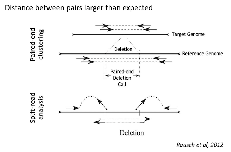
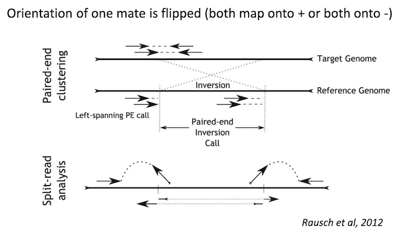
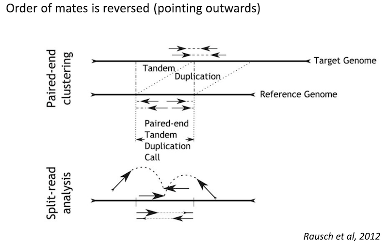
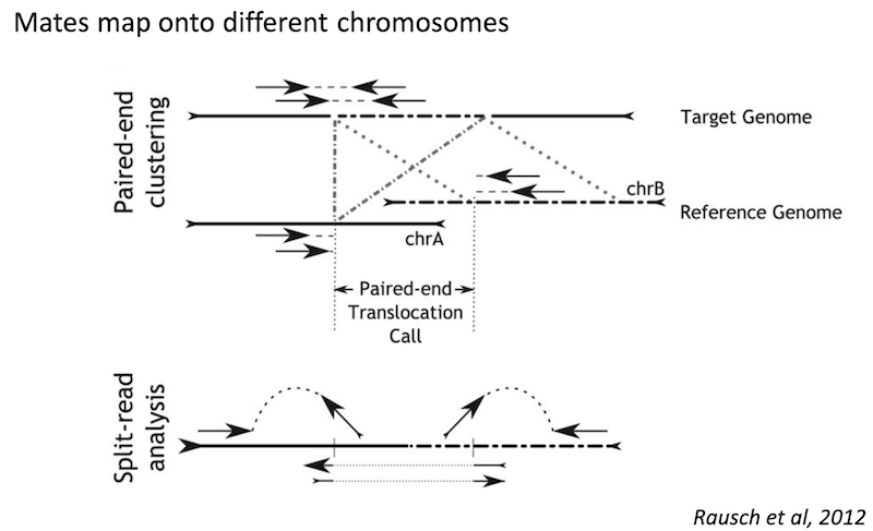
Because structural variants are most often larger than the individual reads we must use different types of read evidence than those used for SNVs and InDels which can be called by simple read alignment. We use three types of read evidence to discover structural variations: discordant read pairs, split-reads, and read depth.
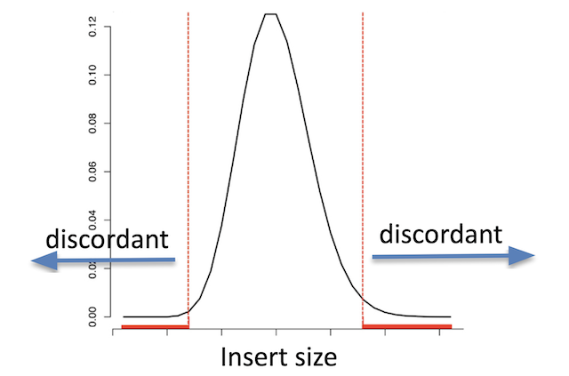
Discordant read pairs have insert sizes that fall significantly outside the normal distribution of insert sizes.
Insert size distribution
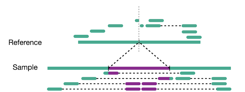
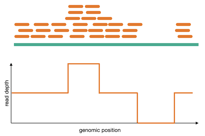
Split reads are those where part of the read aligns to the reference on one side of the breakpoint and the other part of the read aligns to the other side of the deletion breakpoint or to the inserted sequence. Read depth is where increases or decreases in read coverage occur versus the average read coverage of the genome.
Reads aligned to sample genome

Reads aligned to reference genome

Coverage comes in two variants, sequence coverage and physical coverage. Sequence coverage is the number of times a base was read while physical coverage is the number of times a base was read or spanned by paired reads.
Sequence coverage

When there are no paired reads, sequence coverage equals the physical coverage. However, when paired reads are introduced the two coverage metrics can vary widely.
Physcial coverage

Read depth
Read signatures
Deletion read signature
Inversion read signature
Tandem duplication read signature
Translocation read signature
Challenge
What do you think the read signature of an insertion might look like?
Solution
Copy number analysis
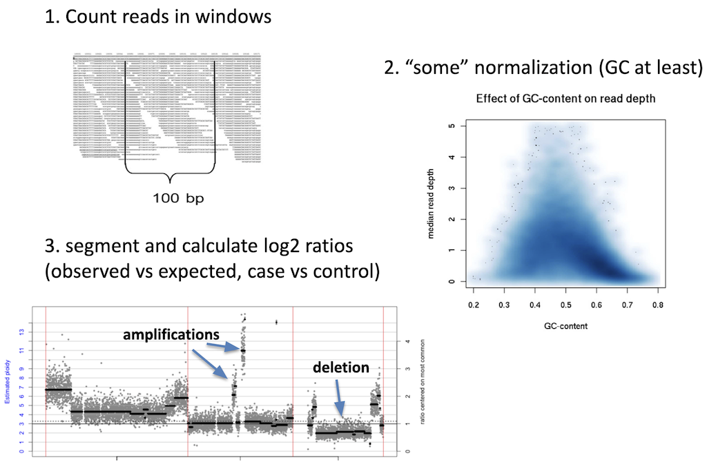
Calling of copy number variation from WGS data is done using read depth, where reads are counted in bins or windows across the entire genome. The counts need to have some normalization applied to them in order to account for sequencing irregularities such as mappability and GC content. These normalized counts can then be converted into their copy number equivalents using a process called segmentation. Read coverage is, however, inheirently noisy. It changes based on genomic regions, DNA quality, and other factors. This makes calling CNVs difficult and is why many CNV callers focus on large variants where it is easier to normalize away smaller confounding changes in read depth.
Caller resolution
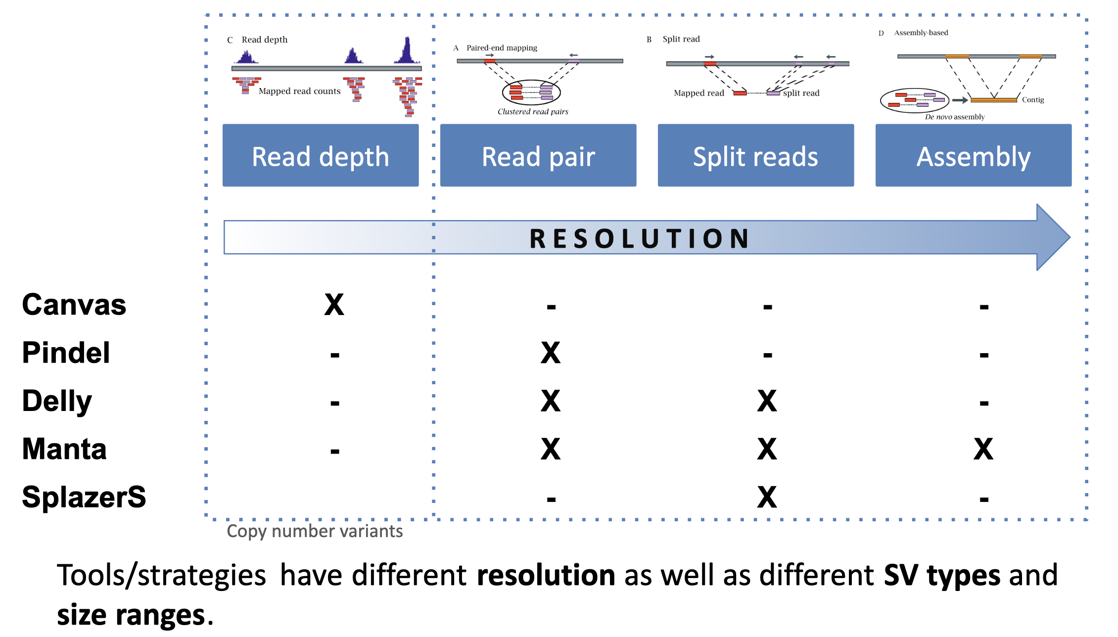
We consider caller resolution to be how likely each algorithm is to determine the exact breakpoints of the SV. Precise location of SV breakpoints is an advantage when merging and regenotyping SVs. Here we are looking at the read signatures we’ve discussed so far: read depth, read pair, and split reads. We also see here another category which is assembly, which in this context means local assembly of the reads from the SV region is used to better determine the breakpoints of the SV.
Caller concordance
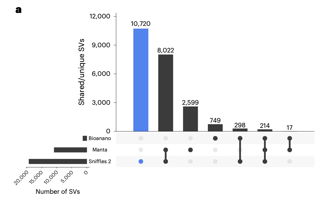
Because SV callers can both use different types of read evidence and apply different weights to the various read signatures, concordance between SV callers is usually quite low in comparison to SNV and InDel variant callers. Concordance between SV calls using different technologies show an even more pronounced lack of concordance.
Key Points
Structural variants are more difficult to identify.
Discovery of SVs usually requires multiple types of read evidence.
There is often significant disagreement between SV callers.
Structural Variation in long reads
Overview
Teaching: 30 min
Exercises: 0 minQuestions
What are the advantages/disadvantages of long reads?
How might we leverage a combination of long and short read data?
Objectives
Investigate how long-read data can improve SV calling.
Long read platforms
The two major platforms in long read sequencing are PacBio and Oxford Nanopore.
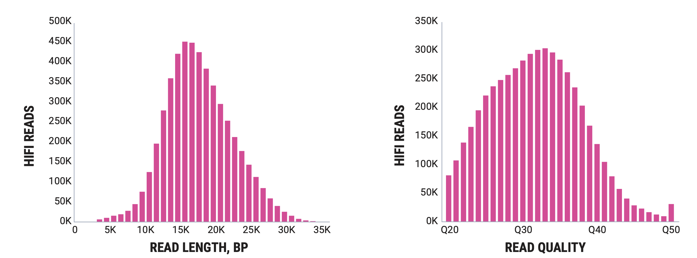
PacBio’s flagship is the Revio, which produces reads in the 5kb to 35kb range with very high accuracy.
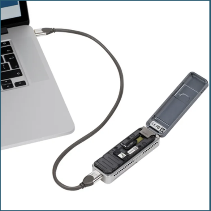
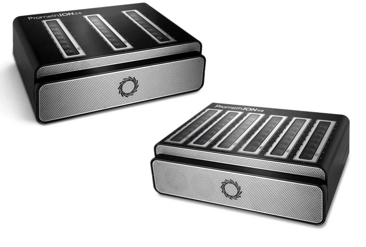
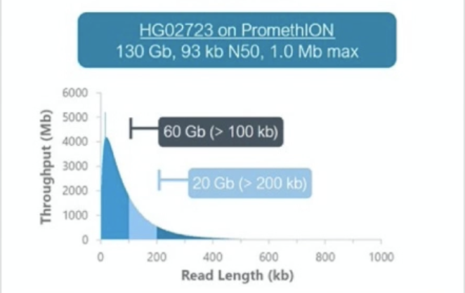
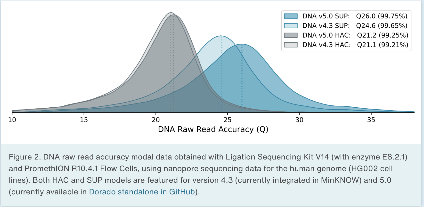
Oxford Nanopore produces sequencers that range in size from the MinION, which is roughly smart phone sized to the PromethION, the high throughput version that we have at NYGC. There are some differences in the read outputs of the various platforms but the MinION has been shown to produce N50 read lengths over 100kb with maximum read lengths greater than 800kb using ONT’s ultra-long sequencing prep. The PromethION can produce even greater N50 values and can produce megabase long reads. Typically these reads are lowe overall base quality than PacBio but ONT has steadily been improving the base quality for their data.
Advantages of long reads
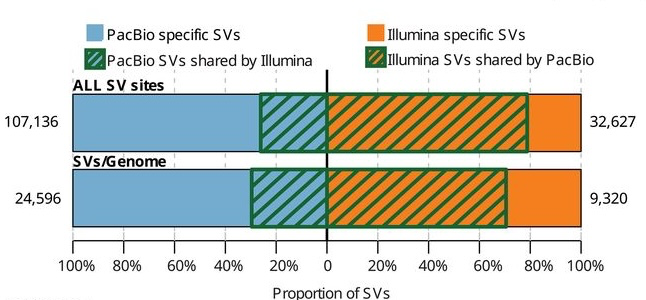
We can call many more SVs using long reads, either by alignment (with enough depth) or assembly (with sufficient assembly quality)1.
Challenge
Why are we able to call more variants with long reads? Why are there Illumina only SVs?
Solution
- Long reads can often be mapped to regions of the genome where short reads fail to map.
Long reads can span larger events making discovery easier and increasing breakpoint accuracy.
- False positives are one possible explaination for Illumina only SVs.
SV calling in long reads
Alignment
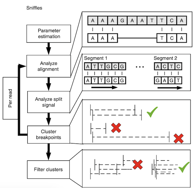
Sniffles uses a three step approach to calling SVs. First it scans the read alignments looking for split reads and inline events. Inline events are insertions and deletions that occur entirely within the read. It puts these SVs into bins and then looks for neighboring bins that can be merged using a repeat aware approach to create these clusters of SV candidates. Each cluster is then re-analyzed and a final determination is made based on read support, expected coverage changes and breakpoint variance.
Assembly
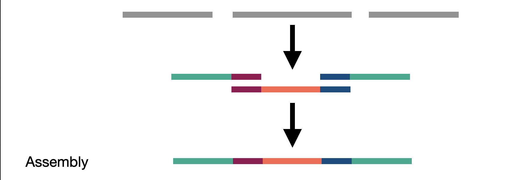
We touched on assembly in the short read section but here we actually refer to whole genome assembly compared to local assembly in short reads. By assembling as much of the genome as possible, including novel insertions, we create a bigger picture of our sample. These assembled fragments, called contigs, can then be aligned to the reference. The contigs act as a sort of ultra-long read as they represent many reads stiched together.

Challenge
Given the previous assembly result and reference sequence, what type of SV are we looking at here?
Drawbacks
- Long read sequencing is becoming more affordable but is still much more expensive than short read
sequencing
SR << LR Alignment << LR Assembly. - Throughput is lower, reducing the turn around time for projects with large numbers of samples.
- Sequencing prep, especially for ultra-long protocols is tedious and difficult to perform consitently.
- Due to cost, we typically don’t sequence samples at as high of depth.
- We are still limited to some extent by the length of our reads and our ablility to span an entire event with one or more reads and some regions of the genome are still very difficult to sequence and align to.
Genotyping LR SVs in SR data
Challenge
Given the section title, what two approaches might we take in creating a hybrid SV call set that uses both long and short reads?
Paragraph
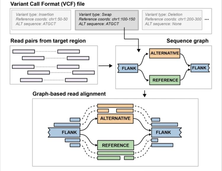
Pangenie
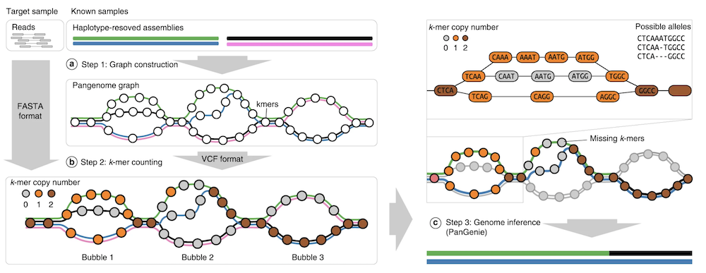
Solution
We can:
- Sequence a number of individuals with long reads and genotype those SV calls in our short read sample set.
- We can leverage existing long read SV callsets and genotype those SVs into out short read sample set.
Question
Does anyone know of any other technologies being used for structural variation?
Callback
Key Points
Long-reads offer significant advantages over short-reads for SV calling.
Genotyping of long-read discovered SVs in short-read data allows for some scalability.
SV Exercises
Overview
Teaching: 0 min
Exercises: 120 minQuestions
How do the calls from short read data compare to those from the long read data?
How do the
Objectives
Align long read data with minimap2
Call SVs in short and long read data
Regenotype LR SVs in a short read data set
Exercises
- Run manta on our SR data for chromosomes 1, 6, and 20
- Run minimap2 on chromosome 20
- Run samtools merge for LR data
- Run sniffles on merged LR bam
Before we really start
Super fun exercise
cd
wget https://github.com/arq5x/bedtools2/releases/download/v2.31.0/bedtools.static
chmod a+x bedtools.static
mv bedtools.static miniconda3/envs/siw/bin/bedtools
First
We’ll make our output directory and change our current directory to it.
mkdir /workshop/output/sv
cd /workshop/output/sv
Manta
There are two steps to running manta on our data. First, we tell Manta what the
inputs are by running configManta.py.
Relevant files - don’t try to execute this, it is just to help you understand what files you need.
_BAM_ -> /data/alignment/combined/NA12878.dedup.bam

_REF_ -> /data/alignment/references/GRCh38_1000genomes/GRCh38_full_analysis_set_plus_decoy_hla.fa
Run the following code blocks one at a time.
/software/manta-1.6.0.centos6_x86_64/bin/configManta.py \
 --bam _BAM_ \
 --referenceFasta _REF_ \
 --runDir _OUT_
./_OUT_/runWorkflow.py \
 --mode local \
 --jobs 8 \
 --memGb unlimited
Challenge
Run manta on NA12878’s parents (NA12891 and NA12892)
ls -lh _OUT_/results/variants/diploidSV.vcf.gz
-rw-r--r-- 1 student student 137K Aug 27 22:54 manta_NA12878/results/variants/diploidSV.vcf.gz
-rw-r--r-- 1 student student 141K Aug 27 23:04 manta_NA12891/results/variants/diploidSV.vcf.gz
-rw-rw-r-- 1 student student 141K Aug 27 23:07 manta_NA12892/results/variants/diploidSV.vcf.gz
Note - data compression
Storing the raw text of our analyses is very inefficient so we often compress our data using data compression programs (gzip, bgzip). This is comes at a cost of convenience though, we can’t use our “normal” tools (cat, less, grep) to access these files in the same way we couldn’t use less to read our BAM files yesterday. However, many tools come with an equivalent for compressed file usage - zcat, zless, zgrep.
Minimap2
Challenge
If we take the first 1000 lines of a fastq file how many reads do we get?
zcat /data/SV/long_read/inputs/NA12878_NRHG.chr20.fq.gz \
| head -n 20000 \
| minimap2 \
    -ayYL \
    --MD \
    --cs \
    -z 600,200 \
    -x map-ont \
    -t 8 \
    -R "@RG\tID:NA12878\tSM:NA12878\tPL:ONT\tPU:PromethION" \
    /data/alignment/references/GRCh38_1000genomes/GRCh38_full_analysis_set_plus_decoy_hla.mmi \
    /dev/stdin \
| samtools \
    sort \
    -M \
    -m 4G \
    -O bam \
> NA12878.minimap2.bam
Flags
- Minimap
- -a : output in the SAM format
- -y : Copy input FASTA/Q comments to output
- -Y : use soft clipping for supplementary alignments
- -L : write CIGAR with >65535 ops at the CG tag
- –MD : output the MD tag
- –cs : output the cs tag
- -z : Z-drop score and inversion Z-drop score
- -x : preset
- -t : number of threads
- -R : SAM read group line
- Samtools
- -M : Use minimiser for clustering unaligned/unplaced reads
- -m : Set maximum memory per thread
- -O : Specify output format
Sniffles
sniffles \
 --threads 8 \
 --input /data/SV/long_read/minimap2/NA12878_NRHG.minimap2.chr1-6-20.bam \
 --vcf NA12878_NRHG.sniffles.vcf
Regenotyping
Another super fun exercise
We need to make a copy of a file and change some of its contents.
cp /data/SV/inputs/NA12878.paragraph_manifest.txt .

vi NA12878.paragraph_manifest.txt
Change
/data/SV/bams/NA12878.chr1-6-20.bamto/data/alignment/combined/NA12878.dedup.bam.
cat
id	path	depth	read length	sex
NA12878	/data/alignment/combined/NA12878.dedup.bam	33.94	150	F
Relevant files - don’t try to execute this, it is just to help you understand what files you need.
_VCF_ -> /data/SV/inputs/HGSVC_NA12878.chr1-6-20.vcf.gz

_MANIFEST_ -> ./NA12878.paragraph_manifest.txt

_REF_ -> /data/alignment/references/GRCh38_1000genomes/GRCh38_full_analysis_set_plus_decoy_hla.fa
~/paragraph-v2.4a/bin/multigrmpy.py \
 -i _VCF_ \
 -m _MANIFEST_ \
 -r _REF_ \
 -o _OUT_ \
 --threads 8 \
 -M 400
Secondary challenges
Manta
How many variants do we call using manta?
Solution
zgrep -vc "^#"What is the breakdown by type?
Sniffles
How many variants do we call using sniffles?
Solution
zgrep -vc "^#" NA12878_NRHG.sniffles.vcf.gz4209What is the breakdown by type?
Solution
zgrep -v "^#" NA12878_NRHG.sniffles.vcf.gz | cut -f 8 | cut -f 2 -d ";" | sort | uniq -c11 SVTYPE=BND 1727 SVTYPE=DEL 1 SVTYPE=DUP 2464 SVTYPE=INS 6 SVTYPE=INVDiscussion
Key Points
Cancer Genomics
Overview
Teaching: 2h min
Exercises: 3h minQuestions
Objectives
Open your terminal
To start we will open a terminal.
- Go to the link given to you at the workshop
- Paste the notebook link next to your name into your browser
- Select “Terminal” from the “JupyterLab” launcher (or blue button with a plus in the upper left corner)
- After you have done this put up a green sticky not if you see a flashing box next to a
$
Slides
You can view Nico’s talk here
Generate somatic variant calls with Mutect2
Mutect2 is a somatic mutation caller in the Genome Analysis Toolkit (GATK), designed for detecting single-nucleotide variants (SNVs) and INDELs (insertions and deletions) in cancer genomes. The input for Mutect2 includes preprocessed alignment files (CRAM files). The CRAMs include sequencing reads that have been aligned to a reference genome, sorted, duplicate-marked, and base quality score recalibrated. Mutect2 can call variants from paired tumor and normal sample CRAM files, and also has a tumor-only mode. Mutect2 uses the matched normal to additionally exclude rare germline variation not captured by the germline resource and individual-specific artifacts.
Executing Mutect2
In this example Mutect2 will be run in a few intervals. This will speed up a minature test run of a Mutect2 command. In reality you might decide to restrict Mutect2 to the WGS calling regions recommended in the Mutect2 resource bundle.
# create a BED file of chr22 intervals to do a fast test run
cat \
  /data/cancer_genomics/allSitesVariant.bed \
  | grep "^chr22" \
  > ~/workspace/output/allSitesVariant.chr22.bed

# run Mutect2 calling command
gatk Mutect2 \
  -R /data/cancer_genomics/GRCh38_full_analysis_set_plus_decoy_hla.fa \
  --intervals ~/workspace/output/allSitesVariant.chr22.bed \
  -I /data/cancer_genomics/COLO-829_2B.variantRegions.cram \
  -I /data/cancer_genomics/COLO-829BL_1B.variantRegions.cram \
  -O ~/workspace/output/COLO-829_2B--COLO-829_829BL_1B.mutect2.unfiltered.vcf
Going further with Mutect2 runs (this is a slower command not run in the workshop)
Real projects should be filtered for technical artifacts with a Panel of Normals (PON) and with common germline variants. The
--germline-resourceand--panel-of-normalsflags are used if Mutect2 is the tool filtering your somatic calls. In the example below the population allele frequency for the alleles that are not in the germline resource is 0.00003125. Read more in the Mutect2 documentation.gatk Mutect2 \ -R /data/cancer_genomics/GRCh38_full_analysis_set_plus_decoy_hla.fa \ -I /data/cancer_genomics/COLO-829_2B.variantRegions.cram \ -I /data/cancer_genomics/COLO-829BL_1B.variantRegions.cram \ --germline-resource AF_ONLY_GNOMAD.vcf.gz \ --af-of-alleles-not-in-resource 0.00003125 \ --panel-of-normals YOUR_PON.vcf.gz \ -O ~/workspace/output/COLO-829_2B--COLO-829_829BL_1B.mutect2.unfiltered.vcf
Filter somatic variant calls
After calling the variants, we filter out low-quality calls using the FilterMutectCalls tool which applies various filters like minimum variant-supporting read depth and mapping quality to distinguish true somatic mutations from artifacts. The full set of filters is described in the Mutect2 GitHub repository.
Filtering Mutect2 calls
gatk FilterMutectCalls \
  --reference /data/cancer_genomics/GRCh38_full_analysis_set_plus_decoy_hla.fa \
  -V ~/workspace/output/COLO-829_2B--COLO-829_829BL_1B.mutect2.unfiltered.vcf \
  --stats ~/workspace/output/COLO-829_2B--COLO-829_829BL_1B.mutect2.unfiltered.vcf.stats \
  -O ~/workspace/output/COLO-829_2B--COLO-829_829BL_1B.mutect2.vcf
Anatomy of a VCF file & bcftools
What is a VCF?
Variant Call Format (VCF) files are a widely used file format for representing genetic variation, with an official specification maintained by the Global Alliance for Genomics & Health (GA4GH). This organization also maintains the specifications for the SAM, BAM, and CRAM file formats. The VCF specification has evolved over time, and can now represent SNVs, INDELs, structural variants, and copy number variants, as well as any annotations. A large ecosystem of software exists for parsing and manipulating VCFs, the most useful of which is BCFtools.
BCFtools is maintained by the same folks as SAMtools, and shares a lot of underlying code (namely the HTSlib library). For most routine tasks, such as sorting, filtering, annotating, and summarizing, BCFtools provides utilities so you don’t have to worry about your own implementation. For more complicated queries and analysis, you may need to write your own code, or use a command line tool with more sophisticated expressions like vcfexpress.
Another commonly used file format for representing variants is the Mutation Annotation Format (MAF). This format’s origins lie in The Cancer Genome Atlas (TCGA) project. It’s only meant to represent SNVs and INDELs, and the specification is quite rigid with respect to the allowed annotations. However, the data is represented in a convenient tabular format and the maftools R package exists for easy plotting, analysis, and comparison to TCGA.
File structures
Like SAM/BAM files, VCFs are split into two parts: the header, followed by the variant calls.
Exercise: Print the help menu for BCFtools
$ bcftools -h
Exercise: Print just the header with BCFtools, print just the variants with bcftools view
$ # view VCF header
$ bcftools view -h ~/workshop/output/COLO-829_2B--COLO-829_829BL_1B.mutect2.vcf
$ # alternately...
$ bcftools head ~/workshop/output/COLO-829_2B--COLO-829_829BL_1B.mutect2.vcf
$ # view the variant calls
$ bcftools view -H ~/workshop/output/COLO-829_2B--COLO-829_829BL_1B.mutect2.vcf | head
VCFs can contain information about multiple samples. In a cancer context, this is usually the paired tumor and normal, but you can imagine a situation in which we have multiple tumors from the same patient (e.g. a primary and metastasis). Each variant call can be thought of as having two parts, variant-level information (e.g., position, reference allele, impact on gene coding sequence), and more fine-grained sample-level information for a given variant (e.g. VAF, sequencing depth).
Exercise: Filter out the Mutect2 calls with
bcftools filterTypically, we want to filter somatic variants to reduce false positives. The FILTER column indicates the relevant filters for a given variant call. Before filtering, this field is blank or contains just a period (“.”). In the earlier filtering step, Mutect2 “soft-filtered” the calls. That is, it filled in the FILTER column for us, but did not yet remove the calls. Sometimes it’s helpful to inspect these flagged calls to debug some downstream issue. To “hard filter”, we want to only keep calls with a PASS in the FILTER column.
Solution
bcftools filter -i "FILTER='PASS'" \
-o ~/workshop/output/COLO-829_2B--COLO-829_829BL_1B.mutect2.pass.vcf \
~/workshop/output/COLO-829_2B--COLO-829_829BL_1B.mutect2.vcf
Note: bcftools filter can also utilize other fields for filtering (e.g. VAF). Read more about filtering expressions here.
The INFO field contains variant level annotations such as gene impact and population frequency. These are typically added by tools such as Ensembl VEP, or bcftools annotate.
Each annotation should have a corresponding entry in the header indicating how the annotation should be parsed for bcftools and other tools (e.g. python’s Pysam or R’s VariantAnnotation), and a plaintext description for you, the user.
The FORMAT column describes the order of sample-level annotations. Each sample is given a column after the FORMAT column, with the order described in FORMAT, and each annotation detailed in the header.
Exercise: What samples are contained in the Mutect2 VCF?
Hint
Try using
bcftools head
Finally, the reference genome contigs used in variant calling are also listed in the header.
Bgzip and tabix indexing
Tabix: fast retrieval of sequence features from generic TAB-delimited files
Sort the Mutect2 VCF, bgzip, and tabix-index VCF with bcftools sort, bgzip, and tabix
Oftentimes, we want to access variants based on their position in the genome. Doing this in a reasonable amount of time requires an index. BCFtools comes with the utilities bgzip and tabix for accomplishing this. Bgzip implements a modified version of the gzip compression algorithm, compressing the data in blocks of a predetermined size. These bgzipped files are perfectly standards-compliant gzip files and will still work with zcat/gunzip/etc. Tabix is a general purpose algorithm for indexing coordinate-sorted genomic coordinate data in tabular format that relies on bgzip compression to work.
Solution
bcftools sort \
-o ~/workshop/output/COLO-829_2B--COLO-829_829BL_1B.mutect2.pass.sorted.vcf \
~/workshop/output/COLO-829_2B--COLO-829_829BL_1B.mutect2.pass.vcf
bgzip ~/workshop/output/COLO-829_2B--COLO-829_829BL_1B.mutect2.pass.sorted.vcf
tabix ~/workshop/output/COLO-829_2B--COLO-829_829BL_1B.mutect2.pass.sorted.vcf.gz

# Shorter answer (done in a single short bcftools command)

bcftools sort \
-O z -Wtbi \
-o ~/workshop/output/COLO-829_2B--COLO-829_829BL_1B.mutect2.pass.sorted.vcf.gz \
~/workshop/output/COLO-829_2B--COLO-829_829BL_1B.mutect2.pass.vcf
Print the variants overlapping the interval “chr22:10000000-110000000” in the uncompressed VCF with bcftools view. Try the same thing with the bgzipped+indexed VCF
Solution
bcftools view \
~/workshop/output/COLO-829_2B--COLO-829_829BL_1B.mutect2.pass.sorted.vcf.gz \
'chr22:10000000-110000000'
Other BCFtools examples
- isec: perform set operations on multiple VCFs (e.g. intersection, union, set differences)
- merge: merge multiple VCFs
- norm: normalize indel representation, specify how multi-allelic sites should be handled
- NOTE: Normalizing INDELs is required before annotation, and when comparing output from multiple variant callers
- reheader: Rename samples and/or change contigs in the header
- query: Extract information from a VCF in a user-defined format
Extracting variants and plotting the VAF distribution
Extract chromosome, position, and tumor VAF from the VCF. In order to extract the correct VAF values, you’ll need to provide BCFtools with the tumor sample name listed in the header.
Extracting information from VCFs
Solution
# copy a VCF from a bucket
mkdir ~/workshop/data/
gcloud storage cp \
gs://nygc-workshop-2024/cancer_genomics/COLO-829_2B--COLO-829BL_1B.snv.indel.results.v7.annotated.vcf.gz* \
~/workshop/data/

bcftools query \
-s COLO-829_2B \
-f "%CHROM\t%POS\t[%AF]\n" \
~/workshop/data/COLO-829_2B--COLO-829BL_1B.snv.indel.results.v7.annotated.vcf.gz \
> ~/workshop/output/COLO-829_2B--COLO-829BL_1B.vafs.tsv
Plot VAF plot for chr21 and chr22. Identify something different on chr22. (for loop)
Solution (run in R terminal)
# pdf('~/workshop/output/vaf_histogram.pdf') # use lines like these to save to a file when needed)
f = '~/workshop/output/COLO-829_2B--COLO-829BL_1B.vafs.tsv'
x = read.table(f, h=F, stringsAsFactors=F,
               sep='\t', col.names=c('chr', 'pos', 'vaf'))

for (chr in unique(x$chr)) {
   hist(x$vaf[x$chr == chr], breaks=20, main=chr)
}
# dev.off() # use lines like these to save to a file when needed)
What do you think the source of the low VAF variants on chr22 could be?
Inspecting alignments with IGV
Good candidates:
- chr22:22949473 - a straightforward clonal SNV
- chr1:3243220 - a straightforward deletion
- chr2:48028500 - a straightforward insertion
Bad candidates:
- chr22:24,098,035 and chr22:24,098,086 - supporting reads have multiple mismatches, soft-clip on the left
- chr22:29289914-29290094 - Five clustered variants all supported by the same set of reads, with soft-clip on the left. “Group by base at …” is our friend here
- chr22:19132585 - 7bp insertion with flanking mismatches and soft-clipping
Bonus exercise: What organism is the contamination coming from?
Solution
Right-click one of the artifact-supporting reads > Copy read sequence > paste into BLAST
Mutational Signatures (working in Python)
Resources:
- COSMIC SBS signature database
- SigProfilerAssignment documentation
- Paper
- Pre-run test inputs/outputs:
mutational_signatures/pre_run_files
Step-by-step version:
- Create input vcf folder
mkdir -p /home/student/workshop/input_vcfs
mkdir -p /home/student/workshop/output

cp /data/cancer_genomics/COLO-829_2B--COLO-829BL_1B.snv.indel.high_confidence.v7.annotated.vcf \
~/workshop/input_vcfs/

cd ~/workshop/
- Install genome
from SigProfilerMatrixGenerator import install as genInstall

genInstall.install('GRCh38', rsync=False, bash=True)
- Generate mutational spectrum count matrix
from SigProfilerMatrixGenerator.scripts import SigProfilerMatrixGeneratorFunc as matGen

matrices = matGen.SigProfilerMatrixGeneratorFunc("SIW_2025", "GRCh38", "/home/student/workshop/input_vcfs/", plot=True, exome=False, bed_file=None, chrom_based=False, tsb_stat=False, seqInfo=False, cushion=100)
Compare the SBS96 count matrix to the COSMIC database here. Looks closest to SBS7a (UV exposure) (/home/student/workshop/input_vcfs/output/plots/SBS_96_plots_SIW_2025.pdf)
- Deconvolve mutational signatures
from SigProfilerAssignment import Analyzer as Analyze Analyze.cosmic_fit(samples="/home/student/workshop/input_vcfs/output/SBS/SIW_2025.SBS96.all", output="/home/student/workshop/output", input_type="matrix", context_type="96", genome_build="GRCh38") - Look at plots of mutational signatures
(/home/student/workshop/output/Assignment_Solution/Activities/Assignment_Solution_Activity_Plots.pdf)
Solution
SBS5: Unknown clock-like signature SBS7a: UV-light exposure SBS7b: UV-light expsure SBS38: Unknown. Found only in ultraviolet light associated melanomas suggesting potential indirect damage from UV-light.
Cohort-level analysis
Most cancer genomics studies involve the study of a whole cohort of samples, not just one or two. Furthermore, we often want to compare to previously-published data to uncover new biology, and as a way to sanity-check our data – e.g, did something go wrong during the many steps to get from biopsy to variant calls?
To dip our toe into cohort-level analysis, we’ll be using the R maftools package and curated TCGA data from its companion package, TCGAmutations. To start, let’s spin up an interactive R session.
Start an interactive R session
Next, let’s load up the R packages we’ll need. Check what TCGA datasets are available and load up the breast cancer cohort.
Solution
dir.create("~/site-library")
if (!require("BiocManager", quietly = TRUE))
    install.packages("BiocManager", lib="~/site-library")
.libPaths("~/site-library")
library(BiocManager)
BiocManager::install("maftools", lib="~/site-library")
BiocManager::install("PoisonAlien/TCGAmutations", lib="~/site-library")
library(maftools)
library(TCGAmutations)

tcga_available()

brca = tcga_load(study = "BRCA")
In an interactive R session, just typing the variable will print its contents. Let’s check what’s inside our brca variable.
Next, let’s plot a basic summary of the cohort, including the variant type, coding consequences, reference and alternate alleles, tumor mutation burden, and the top 10 most mutated genes.
Solution
# pdf('maf_summary.pdf' # use when you need to make a pdf
plotmafSummary(maf=brca, rmOutlier=TRUE, addStat='median', dashboard=TRUE, titvRaw=FALSE)
# dev.off()
We can expand out the top 10 most mutated genes into an oncoprint (also called an oncoplot), showing distribution of mutations in each sample. Oncoprints can contain information from SNVs and INDELs, but also copy number variants.
Exercise: Generate an oncoprint of the top 10 most mutated genes in the breast cancer cohort
Solution
# pdf('oncoprint.pdf')
oncoplot(maf=brca, top=10)
# dev.off()
It can also be useful to zoom in on specific genes, to understand how the mutations are distributed within the genes – are they clustered in a few “hotspots”?
Exercise: Generate lollipop plots of top 3 most frequently mutated genes in the oncoprint
Solution
#pdf('lollipop.pdf')
lollipopPlot(maf=brca, gene='PIK3CA', AACol=HGVSp_Short, showMutationRate=TRUE)
lollipopPlot(maf=brca, gene='TTN', AACol=’HGVSp_Short’, showMutationRate=TRUE)
lollipopPlot(maf=brca, gene='TP53', AACol=’HGVSp_Short’, showMutationRate=TRUE)
#dev.off()


Notice anything different when comparing the distribution of mutations in TTN versus PIK3CA and TP53? TTN is a very long gene and accumulates mutations by chance. Therefore, mutations in this gene are uniformly distributed, rather than clustered in regions of functional importance. The distribution of mutations in a gene’s coding sequence is a signal utilized in some driver gene discovery tools such as OncodriveCLUST.
As mentioned earlier, it can be helpful to comapre a cohort against previously-published data. Let’s compare this cohort’s tumor mutation burden (TMB) to the rest of TCGA.
Solution
# pdf('tcga_comparison.pdf')
tcgaCompare(maf=brca, cohortName='Workshop', logscale=TRUE, capture_size=50)
# dev.off()
The oncoprint hinted at patterns of mutual exclusivity. We can check this in a more statistically rigorous manner with the somaticInteractions function.
Exercise: Check patterns of co-occurence and mutual exclusivity
Solution
# pdf('interactions.pdf')
somaticInteractions(maf=brca, top=20, pvalue=c(0.05, 0.1))
# dev.off()
Key Points
Bulk RNA differential expression
Overview
Teaching: 60 min
Exercises: 120 minQuestions
How do I normalize a bulk RNA dataset?
How can I summarize the relationship between samples?
How can I compare expression based on biological or technical variables?
How can I visualize the results of this comparison?
How can I prepare differential expression results for input into downstream tools for biological insight?
How can I interpret the results of functional enrichment tools?
Objectives
Apply standard bulk workflow pre-processing methods such as DESeq2 normalization given a gene-sample count matrix.
Execute dimensional reduction (PCA) and corresponding visualization.
Understand design formulas and how to apply them to run differential expression.
Summarize differential expression (DE) results using a heatmap visualization as well as MA and volcano plots.
Interpret data visualizations from the above steps.
Use base R commands to output text files from DE results for input into functional enrichment (ORA/GSEA).
Run ORA/GSEA using a web-based tool, and describe the meaning of the resulting output.
Lecture portion
The workshop will include a lecture component of around one hour before the practical session later on.
Slides for this available here.
About this tutorial
This workflow is based on material from the rnaseqGene page on Bioconductor (link).
This data is from a published dataset of an RNA-Seq experiment on airway smooth muscle (ASM) cell lines. From the abstract:
“Using RNA-Seq, a high-throughput sequencing method, we characterized transcriptomic changes in four primary human ASM cell lines that were treated with dexamethasone - a potent synthetic glucocorticoid (1 micromolar for 18 hours).”
Citation:
Himes BE, Jiang X, Wagner P, Hu R, Wang Q, Klanderman B, Whitaker RM, Duan Q, Lasky-Su J, Nikolos C, Jester W, Johnson M, Panettieri R Jr, Tantisira KG, Weiss ST, Lu Q. “RNA-Seq Transcriptome Profiling Identifies CRISPLD2 as a Glucocorticoid Responsive Gene that Modulates Cytokine Function in Airway Smooth Muscle Cells.” PLoS One. 2014 Jun 13;9(6):e99625. PMID: 24926665. GEO: GSE52778
DOI link here.
Setting up to run this tutorial
Open Launcher.
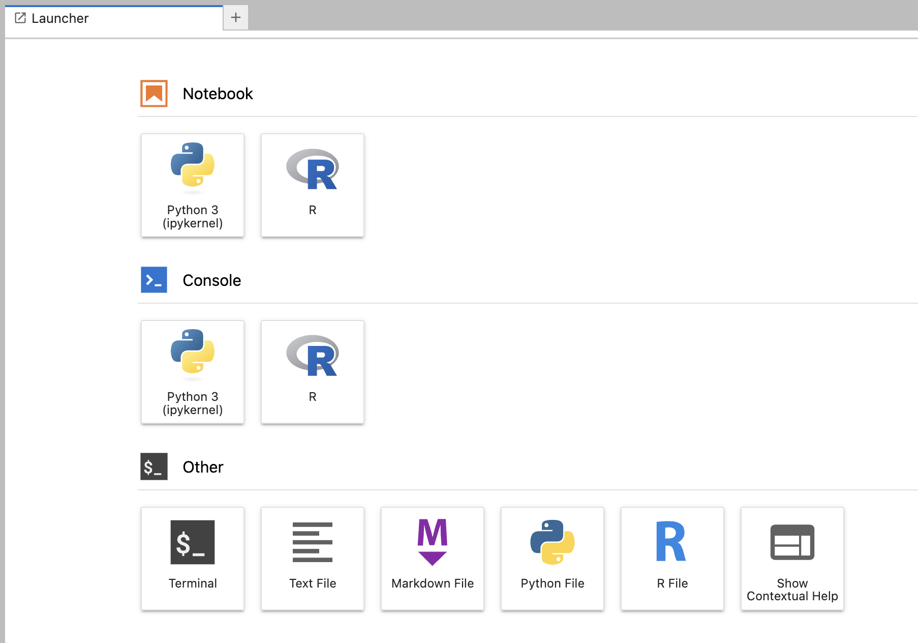
Go to “R” under “Notebook”.
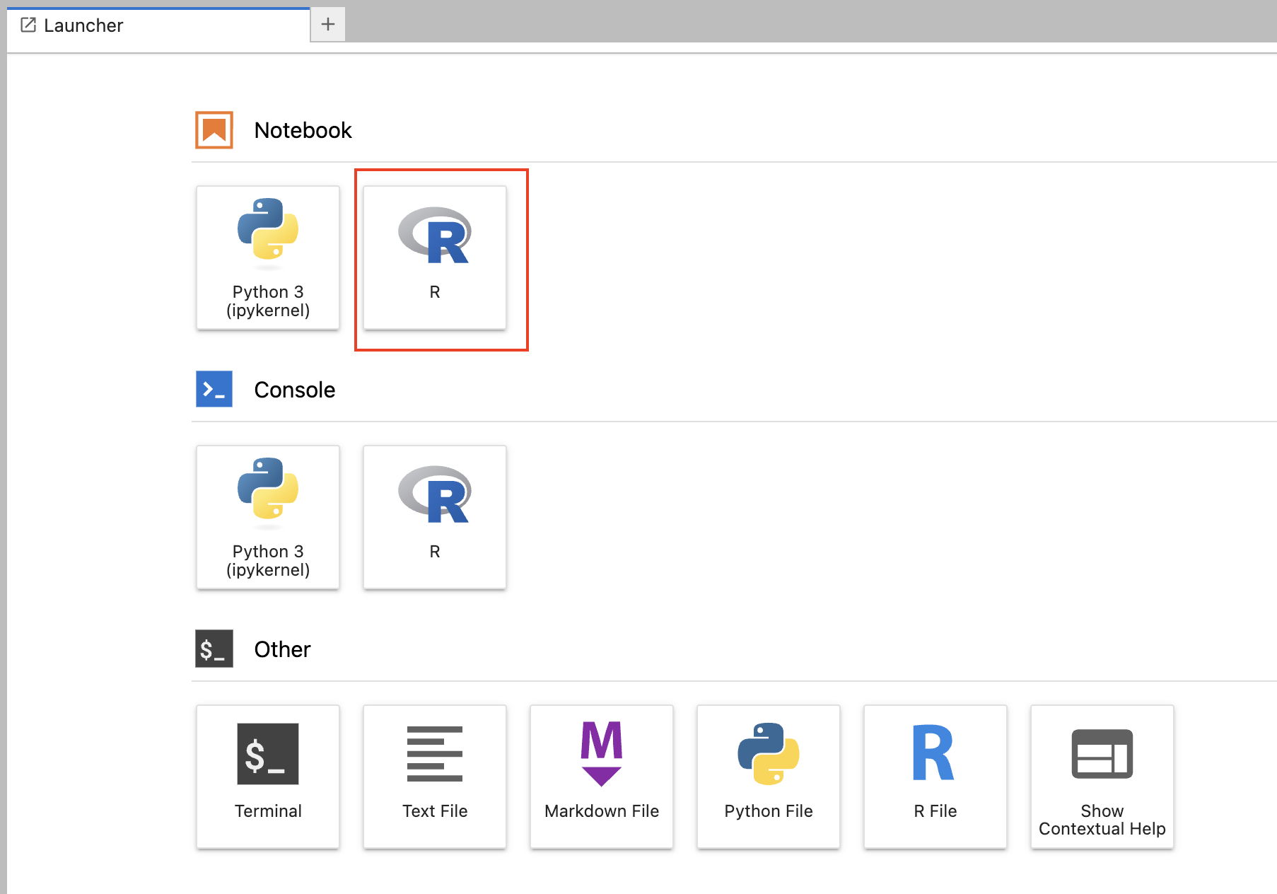

Press the “+” at the top to open another tab.

This time, go to “Other”, then “Terminal”.
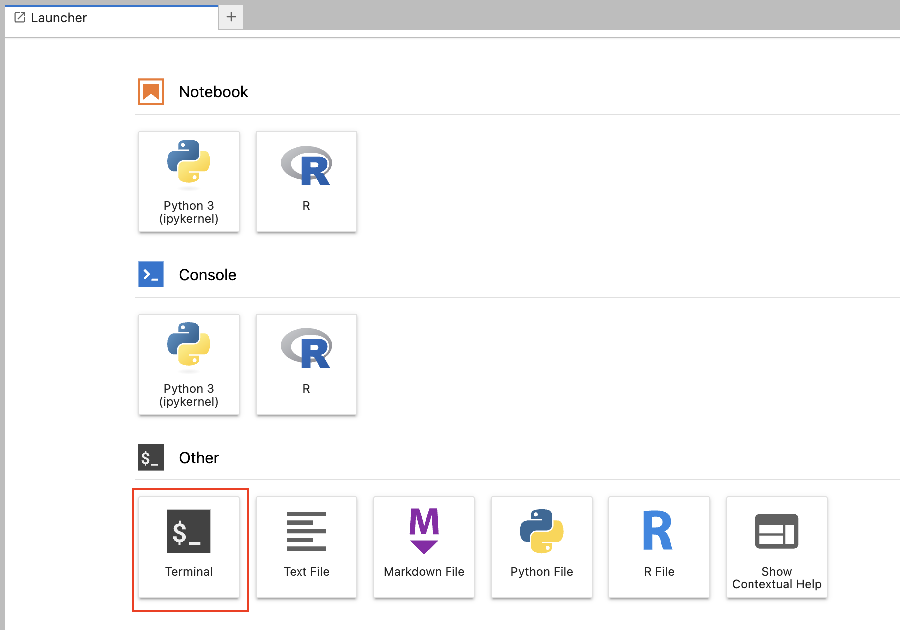

Locating the data on the file system
This section will be run in the “Terminal” tab.
The data has already been downloaded, and is in CSV format for easy reading into R.
The main files we will be working with today are a gene x sample count matrix, and a metadata file with design information for the samples.
Data is available in this directory:
/data/RNA/bulk
If we list that path like so:
ls /data/RNA/bulk
We find the following files:
airway_raw_counts.csv.gz
airway_sample_metadata.csv
To list the files with their full paths, we can use *.
ls /data/RNA/bulk/*
/data/RNA/bulk/airway_raw_counts.csv.gz /data/RNA/bulk/airway_sample_metadata.csv
Bulk RNA differential expression workflow in R with DESeq2
The following will all be run in the R notebook tab.
However, let’s also leave the Terminal tab open for later.
Load libraries.
Load all the libraries you will need for this tutorial using the library command. Today we will load DESeq2, ggplot2, and pheatmap.
library(DESeq2)
library(ggplot2)
library(pheatmap)
Reading in files and basic data exploration.
First, before we read anything into R, what is the full path to the raw counts file?
Solution
/data/RNA/bulk/airway_raw_counts.csv.gz
Use this to read into R using the read.csv command.
Let’s read the help message for this command.
?read.csv
Main argument here is file. Let’s try filling in the path from above.
Solution
read.csv(file=/data/RNA/bulk/airway_raw_counts.csv.gz)Error in parse(text = x, srcfile = src): <text>:1:15: unexpected '/' 1: read.csv(file=/ ^Traceback:
Oops, let’s fix that.
Solution
read.csv(file="/data/RNA/bulk/airway_raw_counts.csv.gz")A data.frame: 63677 × 9 gene_id SRR1039508 SRR1039509 SRR1039512 SRR1039513 SRR1039516 SRR1039517 SRR1039520 SRR1039521 <chr> <int> <int> <int> <int> <int> <int> <int> <int> ENSG00000000003 679 448 873 408 1138 1047 770 572 ENSG00000000005 0 0 0 0 0 0 0 0 ENSG00000000419 467 515 621 365 587 799 417 508 ENSG00000000457 260 211 263 164 245 331 233 229 ENSG00000000460 60 55 40 35 78 63 76 60 ENSG00000000938 0 0 2 0 1 0 0 0 ENSG00000000971 3251 3679 6177 4252 6721 11027 5176 7995 ENSG00000001036 1433 1062 1733 881 1424 1439 1359 1109 ENSG00000001084 519 380 595 493 820 714 696 704 ENSG00000001167 394 236 464 175 658 584 360 269 ... ENSG00000273484 0 0 0 0 0 0 0 0 ENSG00000273485 2 3 1 1 1 1 1 0 ENSG00000273486 14 11 25 8 20 32 12 11 ENSG00000273487 5 9 4 11 10 10 4 10 ENSG00000273488 7 5 8 3 8 16 11 14 ENSG00000273489 0 0 0 1 0 1 0 0 ENSG00000273490 0 0 0 0 0 0 0 0 ENSG00000273491 0 0 0 0 0 0 0 0 ENSG00000273492 0 0 1 0 0 0 0 0 ENSG00000273493 0 0 0 0 1 0 0 0
Looks like we just read in as standard input/output, rather than saving to an object.
Let’s save the result of this command in an object called raw.counts.
Solution
raw.counts = read.csv(file="/data/RNA/bulk/airway_raw_counts.csv.gz")
Use the head command to look at the first few lines.
head(raw.counts)
          gene_id SRR1039508 SRR1039509 SRR1039512 SRR1039513 SRR1039516
1 ENSG00000000003        679        448        873        408       1138
2 ENSG00000000005          0          0          0          0          0
3 ENSG00000000419        467        515        621        365        587
4 ENSG00000000457        260        211        263        164        245
5 ENSG00000000460         60         55         40         35         78
6 ENSG00000000938          0          0          2          0          1
  SRR1039517 SRR1039520 SRR1039521
1       1047        770        572
2          0          0          0
3        799        417        508
4        331        233        229
5         63         76         60
6          0          0          0
Looks like the first column is the gene ids.
It would be better if we could read in such that it would automatically make those the row names, so that all the values in the table could be numeric.
Let’s look at the read.csv help message again to see if there is a way to do that.
?read.csv
If we scroll down we find the following:
row.names: a vector of row names.  This can be a vector giving the
          actual row names, or a single number giving the column of the
          table which contains the row names, or character string
          giving the name of the table column containing the row names.
Let’s use this argument to read in the file again using read.csv, this time taking the first column as the row names.
Solution
raw.counts = read.csv(file="/data/RNA/bulk/airway_raw_counts.csv.gz",row.names=1)
Look at the first few lines of raw.counts again.
head(raw.counts)
                SRR1039508 SRR1039509 SRR1039512 SRR1039513 SRR1039516
ENSG00000000003        679        448        873        408       1138
ENSG00000000005          0          0          0          0          0
ENSG00000000419        467        515        621        365        587
ENSG00000000457        260        211        263        164        245
ENSG00000000460         60         55         40         35         78
ENSG00000000938          0          0          2          0          1
                SRR1039517 SRR1039520 SRR1039521
ENSG00000000003       1047        770        572
ENSG00000000005          0          0          0
ENSG00000000419        799        417        508
ENSG00000000457        331        233        229
ENSG00000000460         63         76         60
ENSG00000000938          0          0          0
Looks good! Think we are ready to proceed with this object now.
Check how many rows there are.
nrow(raw.counts)
[1] 63677
So, we have 63,677 genes, and 8 samples (as we saw when we did head).
Next, read in the file with the study design.
Remember path to this file is:
/data/RNA/bulk/airway_sample_metadata.csv
We can once again use the csv command, and take the first column as row names.
Read into an object called expdesign.
Solution
expdesign = read.csv(file="/data/RNA/bulk/airway_sample_metadata.csv",row.names=1)
Look at the object.
expdesign
              cell   dex avgLength
SRR1039508  N61311 untrt       126
SRR1039509  N61311   trt       126
SRR1039512 N052611 untrt       126
SRR1039513 N052611   trt        87
SRR1039516 N080611 untrt       120
SRR1039517 N080611   trt       126
SRR1039520 N061011 untrt       101
SRR1039521 N061011   trt        98
We are mainly interested in columns cell (says which of the four cell lines the sample is) and dex (says whether or not the sample had drug treatment) here.
Making a DESeq object using DESeq2
We are going to take the raw counts matrix, and the experimental design matrix, and make a special type of object called a DESeqDataSet.
We are going to use a function DESeqDataSetFromMatrix, from the DESeq2 library that we already loaded, to do this.
Let’s view the help message for that function.
?DESeqDataSetFromMatrix
Start of the help message looks like this:
DESeqDataSetFromMatrix(
       countData,
       colData,
       design,
       tidy = FALSE,
       ignoreRank = FALSE,
       ...
     )
We also find the following if we scroll down to the example:
countData <- matrix(1:100,ncol=4)
condition <- factor(c("A","A","B","B"))
dds <- DESeqDataSetFromMatrix(countData, DataFrame(condition), ~ condition)
If we explicitly stated the arguments in the example (and named the objects less confusingly), it would look like this:
mycounts = matrix(1:100,ncol=4)
group = factor(c("A","A","B","B"))
expdesign_example = data.frame(condition = group)
#expdesign_example now looks like this:
#  condition
#1         A
#2         A
#3         B
#4         B
dds = DESeqDataSetFromMatrix(countData = mycounts,
  colData = expdesign_example,
  design = ~condition)
Let’s run this for our data set, but using raw.counts as the count matrix and expdesign as the design matrix.
For the design, let’s look at the column names of expdesign again.
colnames(expdesign)
[1] "cell" "dex" "avgLength"
Here, we want to include both the cell line (cell) and treatment status (dex) in the design.
Save to an object called myDESeqObject.
Solution
myDESeqObject = DESeqDataSetFromMatrix(countData = raw.counts,
  colData = expdesign,
  design = cell,dex)
Error: object 'dex' not found
Oops, looks like we did something wrong.
Should we be putting cell and dex in quotes maybe? That worked the last time we got this kind of error.
Solution
myDESeqObject = DESeqDataSetFromMatrix(countData = raw.counts,
  colData = expdesign,
  design = c("cell","dex"))
Error in DESeqDataSet(se, design = design, ignoreRank) : 'design' should be a formula or a matrix
Hm, still not right.
I think what we are looking for is a design formula here.
If you search for how to make a design formula, you can find this guide, where we seem to see the following rules:
- Design formula should always start with
~. - If more than one variable, put a
+in between. - Nothing in quotes.
For example, their formula for the variables diet and sex was this:
~diet + sex
Let’s see if we can finally fix our command to properly set the design to include cell and dex here.
Solution
myDESeqObject = DESeqDataSetFromMatrix(countData = raw.counts,
  colData = expdesign,
  design = ~cell + dex)
When we run the above, we get the following output:
Warning message:
In DESeqDataSet(se, design = design, ignoreRank) :
some variables in design formula are characters, converting to factors
This is just a warning message, doesn’t mean we did anything wrong.
Looks like the command finally ran OK!
Normalization on the DESeq object
We will next run the estimateSizeFactors command on this object, and save the output back to myDESeqObject.
This command prepares the object for the next step, where we normalize the data by library size (total counts).
myDESeqObject = estimateSizeFactors(myDESeqObject)
Next, we will run a normalization method called rlogTransformation (regularized-log transformation) on myDESeqObject, and save to a new object called rlogObject.
Basic syntax for how this works:
transformedObject = transformationCommand(object = oldObject)
Replace transformedObject here with the name we want for the new object, and transformationCommand with rlogTransformation. Here the oldObject is the DESeq object we already made.
Solution
rlogObject = rlogTransformation(object = myDESeqObject)
Let’s also save just the normalized values from rlogObject in a separate object called rlogMatrix.
rlogMatrix = assay(rlogObject)
Principal components analysis (PCA)
We will run DESeq2’s plotPCA function on the object produced by the rlogTransformation command, to create a plot where we can see the relationship between samples by reducing into two dimensions.
Again, let’s view the help message for this function.
?plotPCA
We find the following documentation.
Usage:

     ## S4 method for signature 'DESeqTransform'
     plotPCA(object, intgroup = "condition", ntop = 500, returnData = FALSE)

Arguments:

  object: a ‘DESeqTransform’ object, with data in ‘assay(x)’, produced
          for example by either ‘rlog’ or
          ‘varianceStabilizingTransformation’.

intgroup: interesting groups: a character vector of names in
          ‘colData(x)’ to use for grouping

Examples:

dds <- makeExampleDESeqDataSet(betaSD=1)
vsd <- vst(dds, nsub=500)
plotPCA(vsd)
A more explicitly stated version of the example:
dds = makeExampleDESeqDataSet(betaSD=1)
raw.counts_example = assay(dds)
expdesign_example = colData(dds)
head(raw.counts_example)
expdesign_example
sample1	sample2	sample3	sample4	sample5	sample6	sample7	sample8	sample9	sample10	sample11	sample12
gene1	6	6	2	8	17	2	0	4	17	7	3	10
gene2	27	48	40	26	12	39	7	5	4	14	9	6
gene3	8	7	4	2	1	1	2	21	4	2	9	0
gene4	36	24	41	25	44	25	39	19	8	31	17	62
gene5	22	36	10	28	33	9	55	58	71	12	68	22
gene6	1	12	5	6	15	1	2	0	7	4	0	1

DataFrame with 12 rows and 1 column
         condition
          <factor>
sample1          A
sample2          A
sample3          A
sample4          A
sample5          A
...            ...
sample8          B
sample9          B
sample10         B
sample11         B
sample12         B
dds = DESeqDataSetFromMatrix(countData = raw.counts_example,
    colData = expdesign_example,
    design=~condition)
vsd <- vst(dds, nsub=500)
plotPCA(object = vsd)
We already ran DESeqDataSetFromMatrix, as well as transformation (we ran rlogTransformation instead of vst, but same idea).
So, just need to plug the object from rlogTransformation into plotPCA.
Solution
plotPCA(object = rlogObject)Error in .local(object, ...) : the argument 'intgroup' should specify columns of colData(dds)
In the example, we did not need to explicitly state what variable to color by in the plot, since there was only one (condition).
However here, we have two possible variables , so we need to explicitly state.
In the example, if we had explicitly stated to color by condition, it would look like this.
plotPCA(object = vsd, intgroup = "condition")
Let’s use the same syntax here to try running plotPCA on rlogObject again, this time explicitly stating to color by cell using the intgroup argument.
Solution
plotPCA(object = rlogObject, intgroup = "cell")
Next, repeat but this time color by dex.
Solution
plotPCA(object = rlogObject, intgroup = "dex")
Interpreting the PCA plot
Let’s look at the two plots we made, and answer the following.
- What principal component separates the four different cell lines? Which one separates treated vs. untreated?
- How much variance is explained by each principal component (hint: see axis labels)?
Solution
PC2 separates the four different cell lines. PC1 separates treated vs. untreated.
PC1 explains 39% of the variance. PC2 explains 27% of the variance.
Differential expression testing
Now that we have created the DESeq object, and done some initial data exploration, it is time to run differential expression testing to see which genes are significantly different between conditions (here, drug-treated vs. not drug-treated).
One step we need to run to get these results is the command DESeq. Let’s pull up the help message for this.
?DESeq
Start of this help message:
Usage:

     DESeq(
       object,
       test = c("Wald", "LRT"),
       fitType = c("parametric", "local", "mean", "glmGamPoi"),
       sfType = c("ratio", "poscounts", "iterate"),
       betaPrior,
       full = design(object),
       reduced,
       quiet = FALSE,
       minReplicatesForReplace = 7,
       modelMatrixType,
       useT = FALSE,
       minmu = if (fitType == "glmGamPoi") 1e-06 else 0.5,
       parallel = FALSE,
       BPPARAM = bpparam()
     )

Arguments:

  object: a DESeqDataSet object, see the constructor functions
          ‘DESeqDataSet’, ‘DESeqDataSetFromMatrix’,
          ‘DESeqDataSetFromHTSeqCount’.
Seems like we can just input our DESeqDataSet object to the object argument?
Let’s do that, and save as a new object called dds.
dds = DESeq(object = myDESeqObject)
If all goes well, you should get the following output as the command runs.
using pre-existing size factors
estimating dispersions
gene-wise dispersion estimates
mean-dispersion relationship
final dispersion estimates
fitting model and testing
Next, we will need to run the results function on dds.
Now, pull up the help message for that function.
?results
Usage:

     results(
       object,
       contrast,
       name,
       lfcThreshold = 0,
...)

Arguments:

  object: a DESeqDataSet, on which one of the following functions has
          already been called: ‘DESeq’, ‘nbinomWaldTest’, or
          ‘nbinomLRT’

contrast: this argument specifies what comparison to extract from the
          ‘object’ to build a results table. one of either:

            • a character vector with exactly three elements: the name
              of a factor in the design formula, the name of the
              numerator level for the fold change, and the name of the
              denominator level for the fold change (simplest case)

...

Examples:

     ## Example 1: two-group comparison

     dds <- makeExampleDESeqDataSet(m=4)

     dds <- DESeq(dds)
     res <- results(dds, contrast=c("condition","B","A"))
To highlight the example:
dds <- DESeq(dds)
res <- results(dds, contrast=c("condition","B","A"))
Replace condition, B, and A with the appropriate values for this data set.
We are looking to compare the effect of treatment with the drug.
Let’s look at our experimental design matrix again.
expdesign
              cell   dex avgLength
SRR1039508  N61311 untrt       126
SRR1039509  N61311   trt       126
SRR1039512 N052611 untrt       126
SRR1039513 N052611   trt        87
SRR1039516 N080611 untrt       120
SRR1039517 N080611   trt       126
SRR1039520 N061011 untrt       101
SRR1039521 N061011   trt        98
Filling in the contrast argument to
resultsfrom expdesignSome questions we need to answer here are:
- What is the variable name for drug treatment here?
- What are the two levels of this variable?
- What order should we put these two levels in, if we want untreated to be the baseline?
Solution
- The variable name for drug treatment is
dex.- The two levels are
trtanduntrt.- We should put
trtfirst anduntrtsecond so that the fold-change will be expressed as treated/untreated.
Now that we figured that out, we just need to plug everything into the function.
Output to an object called res.
Solution
res = results(object = dds, contrast = c("dex","trt","untrt"))
Let’s look at the first few rows of the results using head.
head(res)
log2 fold change (MLE): dex trt vs untrt
Wald test p-value: dex trt vs untrt
DataFrame with 6 rows and 6 columns
                  baseMean log2FoldChange     lfcSE      stat      pvalue
                 <numeric>      <numeric> <numeric> <numeric>   <numeric>
ENSG00000000003 708.602170     -0.3812540  0.100654 -3.787752 0.000152016
ENSG00000000005   0.000000             NA        NA        NA          NA
ENSG00000000419 520.297901      0.2068126  0.112219  1.842943 0.065337292
ENSG00000000457 237.163037      0.0379204  0.143445  0.264356 0.791505742
ENSG00000000460  57.932633     -0.0881682  0.287142 -0.307054 0.758801924
ENSG00000000938   0.318098     -1.3782270  3.499873 -0.393793 0.693733530
                      padj
                 <numeric>
ENSG00000000003 0.00128292
ENSG00000000005         NA
ENSG00000000419 0.19646985
ENSG00000000457 0.91141962
ENSG00000000460 0.89500478
ENSG00000000938         NA
Run the following to get an explanation of what each column in this output means.
mcols(res)$description
[1] "mean of normalized counts for all samples"
[2] "log2 fold change (MLE): dex trt vs untrt"
[3] "standard error: dex trt vs untrt"
[4] "Wald statistic: dex trt vs untrt"
[5] "Wald test p-value: dex trt vs untrt"
[6] "BH adjusted p-values"
Ready to start to explore and interpret these results.
Visualizing expression of differentially expressed genes (heatmap)
Use the which function to get the indices (row numbers) of the genes with adjusted p-value < .01 (false discovery rate of 1%).
Then, save as an object called degs.
First, which column index or name contains the adjusted p-values?
Solution
Column "padj", or column number 6.
Then, we will need to extract this column. A few possible ways listed below.
Solution
res$padj
res[,6]
res[,"padj"]
Next, help message for the which command (from base package) gives the following:
Usage:

     which(x, arr.ind = FALSE, useNames = TRUE)
     arrayInd(ind, .dim, .dimnames = NULL, useNames = FALSE)

Arguments:

       x: a ‘logical’ vector or array.  ‘NA’s are allowed and omitted
          (treated as if ‘FALSE’).

Examples:

     which(LETTERS == "R")
..
which(1:10 > 3, arr.ind = TRUE)
So, we just need to add a statement to get only values less than 0.01 from the column.
Solution
degs = which(res$padj < .01)
How many differentially expressed genes do we find?
length(degs)
[1] 2901
Next, let’s subset the normalized expression matrix (rlogMatrix) to only these genes, and output to a new matrix rlogMatrix.degs.
Syntax of matrix subsetting:
mydat.subset = mydat[indices_to_subset,]
Solution
rlogMatrix.degs = rlogMatrix[degs,]
Let’s run the pheatmap command on this matrix to output a heatmap to the console.
pheatmap(object = rlogMatrix.degs)
Error in pheatmap(object = rlogMatrix.degs) :
  argument "mat" is missing, with no default
Well, that’s why we should read the help message! Seems the main argument for the input object to pheatmap is mat, not object.
pheatmap(mat = rlogMatrix.degs)
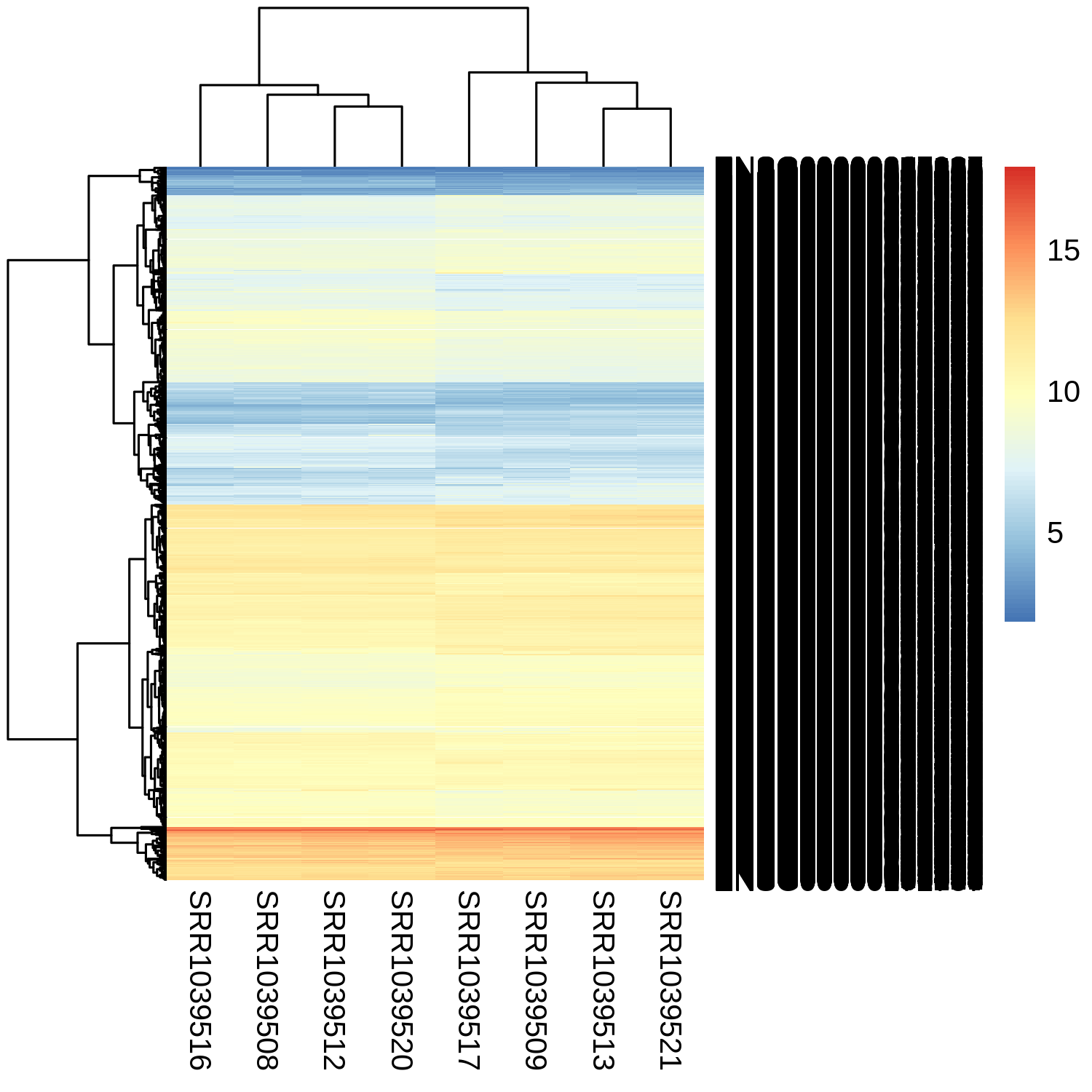
Does not seem super informative!
Let’s look at the pheatmap help message again and see if we can add some arguments to make it better.
?pheatmap
Scrolling down to arguments, we see:
scale: character indicating if the values should be centered and
          scaled in either the row direction or the column direction,
          or none. Corresponding values are ‘"row"’, ‘"column"’ and
          ‘"none"’
Let’s scale across the genes, so by row.
And also this:
show_rownames: boolean specifying if row names are be shown.
Boolean means either TRUE or FALSE. Let’s turn this off.
Solution
pheatmap(mat = rlogMatrix.degs,
    scale="row",
    show_rownames=FALSE)
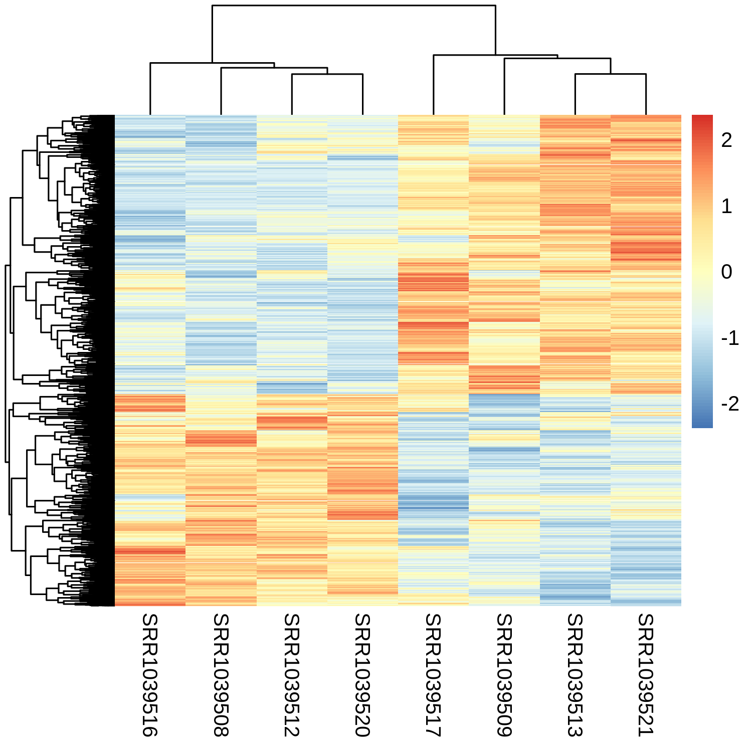
Think we mostly have what we want now.
Except, the “SRR” sample names are not very informative.
It would be good to have an annotation bar at the top of the heatmap that said what cell line each sample is from, and whether it is treated or untreated.
Going back to the pheatmap help message:
annotation_row: data frame that specifies the annotations shown on left
          side of the heatmap. Each row defines the features for a
          specific row. The rows in the data and in the annotation are
          matched using corresponding row names. Note that color
          schemes takes into account if variable is continuous or
          discrete.

annotation_col: similar to annotation_row, but for columns.
We already have a data frame with the annotation we are looking for, so just need to give it as an argument here.
Solution
pheatmap(mat = rlogMatrix.degs,
    scale="row",
    show_rownames=FALSE,
    annotation_row=expdesign)
Error in seq.int(rx[1L], rx[2L], length.out = nb) : 'from' must be a finite number In addition: Warning messages: 1: In min(x) : no non-missing arguments to min; returning Inf 2: In max(x) : no non-missing arguments to max; returning -Inf
Oops - looks like we used the wrong argument. We want to annotate the samples, not the genes.
Solution
pheatmap(mat = rlogMatrix.degs,
    scale="row",
    show_rownames=FALSE,
    annotation_col=expdesign)
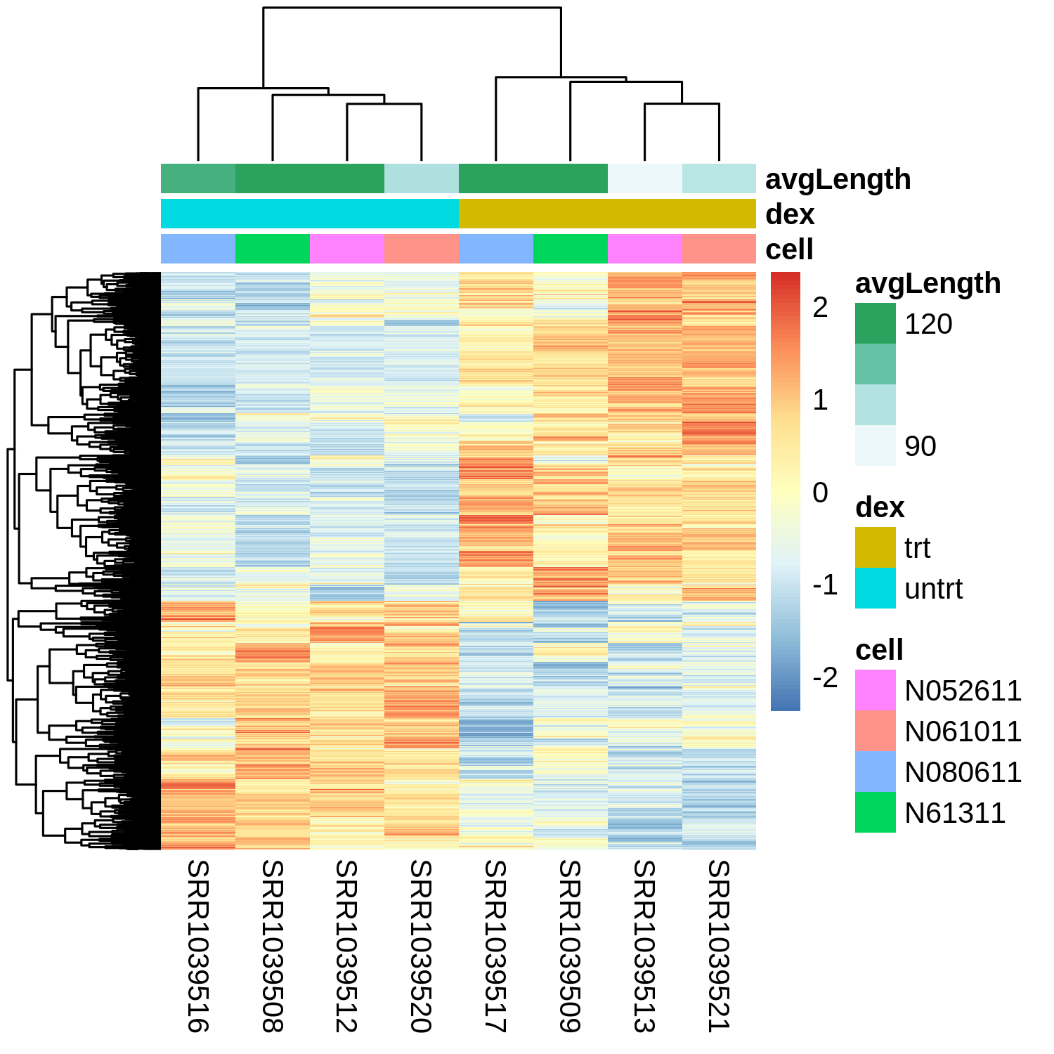
Looks like the samples separate primarily by treatment, as we would expect here since these are the differentially expressed genes.
We also see some variability by cell line, as we would have expected from the PCA plot.
Finally, we see a mix of genes upregulated vs. downregulated in the treated condition.
Visualizing differential expression statistics (scatterplots)
MA plot
In the above section, we only looked at the differentially expressed genes.
However, we may also want to look at patterns in the differential expression results overall, including genes that did not reach significance.
One common summary plot from differential expression is the MA plot.
In this plot, mean expression across samples (baseMean) is compared to log-fold-change, with genes colored by whether or not they meet the significance level we set for adjusted p-value (padj).
Generally for lowly expressed genes, the difference between conditions has to be stronger to create statistically significant results compared to highly expressed genes. The MA plot shows this effect.
DESeq2 has a nice function plotMA that will do this for you (using the output of the results function), and format everything nicely.
Add argument alpha=0.01 to set the adjusted p-value cutoff to 0.01 instead of the default 0.1.
plotMA(object = res,alpha=0.01)
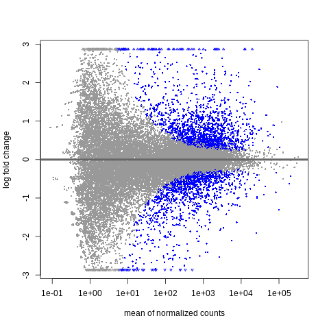
The x-axis here is log10-scaled. The y-axis here is log2(treated/untreated).
The blue dots are for significantly differentially expressed genes (padj < .01).
We find that at low baseMean (closer to 1e+01 or ~10), the magnitude of the log2-fold-change must be very large (often +/-2 or +/- 3, so something like 4-fold or 8-fold difference) for the gene to be significant.
Meanwhile at higher baseMean (say, as we go to 1e+03 or ~1000 reads and above), we find that the magnitude of the log2-fold-change can be much smaller (going down to +/- 0.5, so something like a 1.4-fold difference, or even less).
Volcano plot
Another interesting plot is a volcano plot. This is a plot showing the relationship between the log2-fold-change and the adjusted p-value.
First, extract these two values from res.
Let’s refresh ourselves on what the column names are here.
colnames(res)
[1] "baseMean"       "log2FoldChange" "lfcSE"          "stat"
[5] "pvalue"         "padj"
Extract columns log2FoldChange and padj into objects of the same name.
Solution
log2FoldChange = res$log2FoldChange
padj = res$padj
Plot log2FoldChange on the x-axis and padj on the y-axis.
Solution
plot(log2FoldChange,padj)
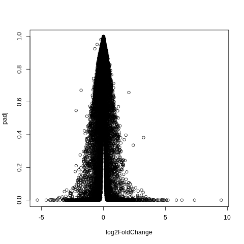
Add argument to make the points smaller.
Argument:
pch="."
Solution
plot(log2FoldChange,padj,pch=".")
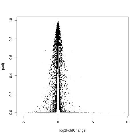
Hm, this still doesn’t look quite right.
If I search for what a volcano plot should look like, I get something closer to this.
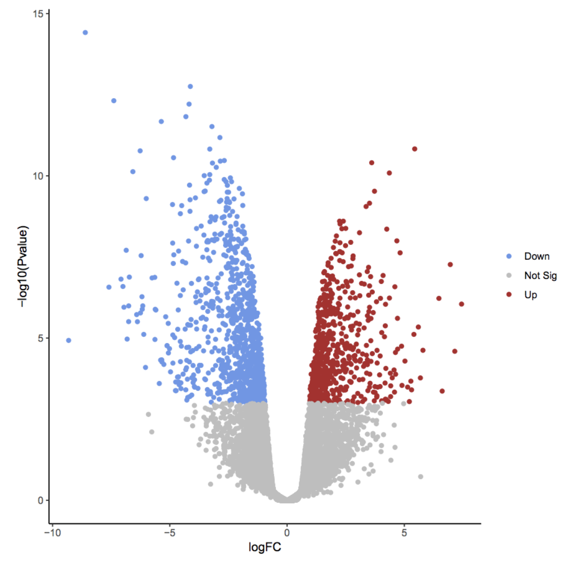
I believe we need to take -log10 of padj.
Let’s do that, and save as padj_transformed.
Then, redo plot using this new variable.
Solution
padj_transformed = -log10(padj)

plot(log2FoldChange,padj_transformed,pch=".")
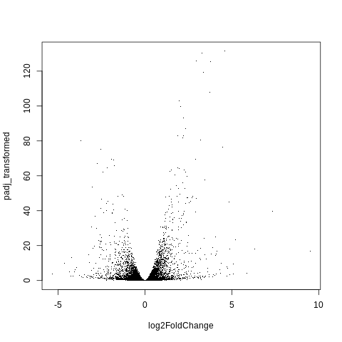
Preparing files for functional enrichment (ORA/GSEA)
Next, we will want to take the results of differential expression testing, and prepare for input into functional enrichment, either over-representation (ORA) or gene set enrichment (GSEA) analysis.
Then, we will import these inputs to a web-based tool called WebGestalt.
In over-representation analysis, the idea is to test whether genes that are significantly differential expressed are enriched for certain categories of genes (gene sets). The input to this is a list of the gene IDs/names for the differentially expressed genes.
In gene set enrichment analysis, genes are ranked by how differential expressed they are, and whether they are upregulated or downregulated. The input to this is a table with the gene IDs/names of all genes, and the test-statistic (here the stat column), ordered by the test-statistic.
Preparing for input into ORA
Here, we will prepare the input for ORA by first getting all the gene IDs into an object called geneids.
These gene IDs are stored in the row names of the results (res), so we can get them out using the rownames function.
Solution
geneids = rownames(res)
Next, subset geneids to just the differentially expressed genes using the previously calculated indices (that we made for the heatmap step).
Syntax to subset an object using previously calculated indices.
x_subset = x[previously_calculated_indices]
Let’s output to an object called geneids.sig.
Solution
geneids.sig = geneids[degs]
Output to a text file called geneids_sig.txt using the writeLines command.
Let’s get the syntax for this command.
?writeLines
Usage:

     writeLines(text, con = stdout(), sep = "\n", useBytes = FALSE)

Arguments:

    text: A character vector

     con: A connection object or a character string.
There is no example in the help message, but I found one on Stack Overflow that may be helpful (paraphrased below).
mywords = c("Hello","World")
output_file = "output.txt"
writeLines(text = mywords, con = output_file)
Let’s run this here.
Solution
output_file = geneids_sig.txt

writeLines(text = geneids.sig, con = output_file)
Error: object 'geneids_sig.txt' not found
Oops, let’s fix.
Solution
output_file = "geneids_sig.txt"

writeLines(text = geneids.sig, con = output_file)
Go to the Terminal tab, and let’s look at this file in more detail.
First, do head and tail.
head geneids_sig.txt
ENSG00000000003
ENSG00000000971
ENSG00000001167
ENSG00000002834
ENSG00000003096
ENSG00000003402
ENSG00000004059
ENSG00000004487
ENSG00000004700
ENSG00000004799
tail geneids_sig.txt
ENSG00000272695
ENSG00000272761
ENSG00000272796
ENSG00000272841
ENSG00000272870
ENSG00000273038
ENSG00000273131
ENSG00000273179
ENSG00000273259
ENSG00000273290
Also check number of lines.
wc -l geneids_sig.txt
2901 geneids_sig.txt
All looks good.
Normally, you would download the file you just created to your laptop, but we may not always have a way to transfer files from the cloud VM to your laptop. So, let’s download the file from the Github for this workshop. Download link here.
Preparing for input into GSEA
Let’s move on to creating the input for GSEA. This will be a data frame with two columns.
gene: The gene ID (already have these for all genes ingeneids)stat: Thestatcolumn from the differential expression results (res)
We will use the data.frame function here.
?data.frame
Examples:

L3 <- LETTERS[1:3]
char <- sample(L3, 10, replace = TRUE)
d <- data.frame(x = 1, y = 1:10, char = char)
Let’s call this data frame gsea.input.
Solution
gsea.input = data.frame(gene = geneids,
    stat = res$stat)
Sort by the stat column.
Solution
order_genes = order(gsea.input$stat)

gsea.input = gsea.input[order_genes,]
Output to a tab-delimited text file gsea_input.txt using the write.table function.
Solution
output_file = "gsea_input.txt"
write.table(x = gsea.input,file=output_file,sep="\t")
Let’s switch over to the Terminal tab and look at this file in more detail.
head gsea_input.txt
"gene"	"stat"
"10923"	"ENSG00000162692"	-19.4160587914648
"14737"	"ENSG00000178695"	-18.8066074036207
"3453"	"ENSG00000107562"	-18.0775817519565
"9240"	"ENSG00000148848"	-18.0580936880167
"8911"	"ENSG00000146250"	-17.7950173361052
"3402"	"ENSG00000106976"	-17.6137734750388
"11121"	"ENSG00000163394"	-17.4484303669187
"5627"	"ENSG00000124766"	-17.1299063626842
"3259"	"ENSG00000105989"	-15.8949963870475
Info on formatting of the file for input into GSEA available here, from the Broad Institute’s documentation.
This says that there should be two columns - one for the feature identifiers (i.e. gene IDs or symbols) and one for the weight of the gene (here, the stat column). But our output has three columns - this is not what we want.
Let’s go back to the R notebook tab and see if we can fix this.
Comparing to the example in the file format documentation, it seems we should do the following:
- Remove the quotation marks.
- Remove the header.
- Remove the first column.
Go back to R and see if we can find arguments in the read.table function to help with this.
?read.table
Arguments:

quote: a logical value (‘TRUE’ or ‘FALSE’) or a numeric vector.  If
          ‘TRUE’, any character or factor columns will be surrounded by
          double quotes.  If a numeric vector, its elements are taken
          as the indices of columns to quote.  In both cases, row and
          column names are quoted if they are written.  If ‘FALSE’,
          nothing is quoted.
row.names: either a logical value indicating whether the row names of
          ‘x’ are to be written along with ‘x’, or a character vector
          of row names to be written.

col.names: either a logical value indicating whether the column names
          of ‘x’ are to be written along with ‘x’, or a character
          vector of column names to be written.  See the section on
          ‘CSV files’ for the meaning of ‘col.names = NA’.
Looks like we need to add a few arguments to get our output formatted correctly.
Let’s output to a new file gsea_input_corrected.txt.
Solution
output_file = "gsea_input_corrected.txt"
write.table(x = gsea.input,file=output_file,sep="\t",row.names=FALSE,col.names=FALSE,quote=FALSE)
Go back to the Terminal tab, and look at this file again.
head gsea_input_corrected.txt
ENSG00000162692	-19.4160587914648
ENSG00000178695	-18.8066074036207
ENSG00000107562	-18.0775817519565
ENSG00000148848	-18.0580936880167
ENSG00000146250	-17.7950173361052
ENSG00000106976	-17.6137734750388
ENSG00000163394	-17.4484303669187
ENSG00000124766	-17.1299063626842
ENSG00000105989	-15.8949963870475
ENSG00000108821	-15.2668170602372
Looks ok - what about tail?
tail gsea_input_corrected.txt
ENSG00000273470	NA
ENSG00000273471	NA
ENSG00000273475	NA
ENSG00000273479	NA
ENSG00000273480	NA
ENSG00000273481	NA
ENSG00000273482	NA
ENSG00000273484	NA
ENSG00000273490	NA
ENSG00000273491	NA
Let’s also check the line count.
wc -l gsea_input_corrected.txt
63677 gsea_input_corrected.txt
Hm - don’t think we should be including genes with an NA for the stat column?
Let’s fix again.
Let’s use grep to remove lines with “NA”, and output to a new file gsea_input_corrected_minus_NA.txt.
Solution
grep -v NA gsea_input_corrected.txt > gsea_input_corrected_minus_NA.txt
Check again.
head gsea_input_corrected_minus_NA.txt
ENSG00000162692	-19.4160587914648
ENSG00000178695	-18.8066074036207
ENSG00000107562	-18.0775817519565
ENSG00000148848	-18.0580936880167
ENSG00000146250	-17.7950173361052
ENSG00000106976	-17.6137734750388
ENSG00000163394	-17.4484303669187
ENSG00000124766	-17.1299063626842
ENSG00000105989	-15.8949963870475
ENSG00000108821	-15.2668170602372
tail gsea_input_corrected_minus_NA.txt
ENSG00000154734	20.2542354089516
ENSG00000125148	20.9292144890544
ENSG00000162614	21.6140905458227
ENSG00000157214	21.968453609644
ENSG00000211445	22.4952633774851
ENSG00000189221	23.6530144138538
ENSG00000101347	24.2347153246759
ENSG00000120129	24.2742584224751
ENSG00000165995	24.7125510867281
ENSG00000152583	24.8561114516005
wc -l gsea_input_corrected_minus_NA.txt
33469 gsea_input_corrected_minus_NA.txt
We now have fewer lines, because we removed the lines for the genes with an “NA” in the stat column.
You can download a copy of this file here.
Running functional enrichment (ORA/GSEA)
Let’s head to the website WebGestalt.
Run ORA
Click “Click to upload” next to “Upload ID List”.
Upload geneids_sig.txt.
For the reference set, select “genome protein-coding”.

In advanced parameters, switch from top 10 to FDR 0.05.
Let’s look at the results!
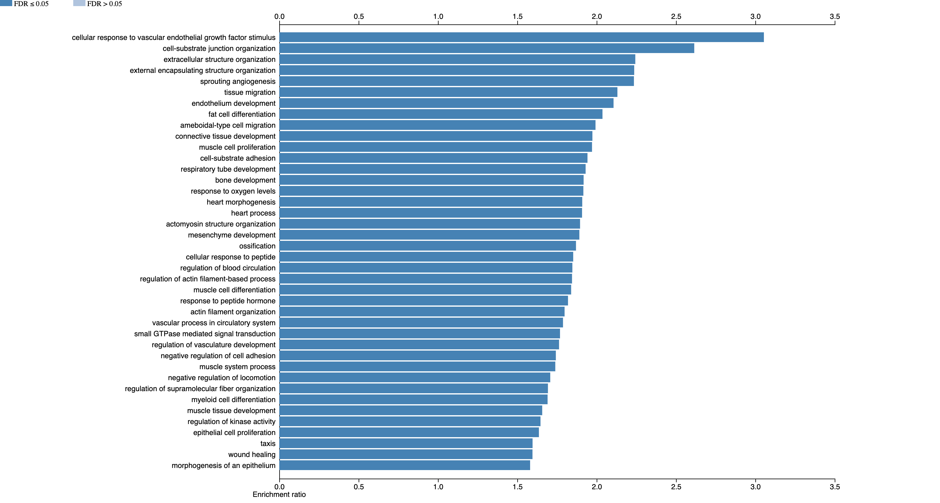
Let’s scroll down and click on “response to oxygen levels”, as this seems pretty relevant for an airway dataset.
We can scroll through and look at the genes that are in this gene set, that are differentially expressed.
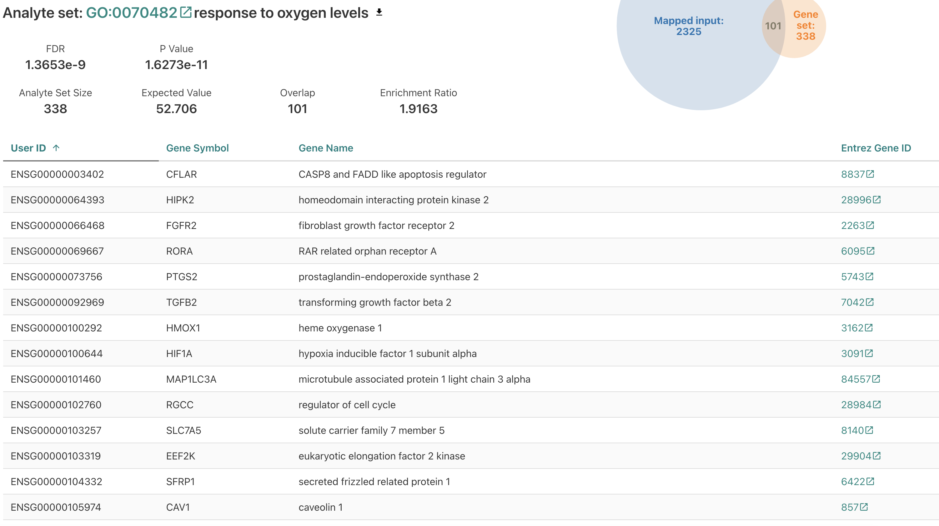
Run GSEA.
Let’s move on to running gene set enrichment analysis (GSEA).
For the tab at the top, switch to “Gene Set Enrichment Analysis”.
Switch back the functional database to the same as before (geneontology, Biological Process noRedundant).
This time, upload gsea_input_corrected_minus_NA.txt.
Also reset the advanced parameters to select based on FDR of 0.05 rather than the top 10 again.
We get the following error message.

Turns out, this is as simple as renaming the file!
Let’s change the file suffix to “.rnk” instead of “.txt” (rename the file).
Below is shown how to do this using Mac’s Finder program - you can do this however you would normally for your system.
Now, go back and redo all of the above, but input gsea_input_corrected_minus_NA.rnk.
This time it should work, and output something like the following:

Hm - fewer categories than we might have expected?
Let’s redo, but change functional database to pathway = Kegg.
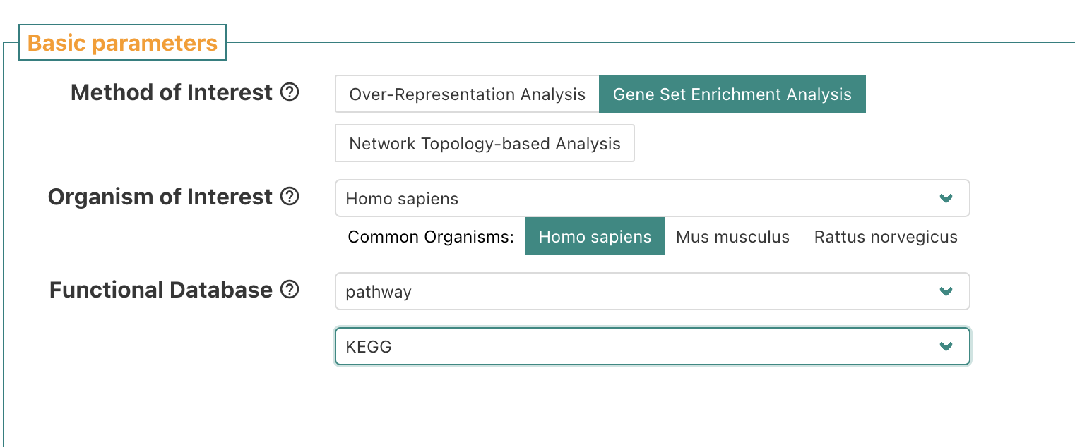

Click on autophagy.
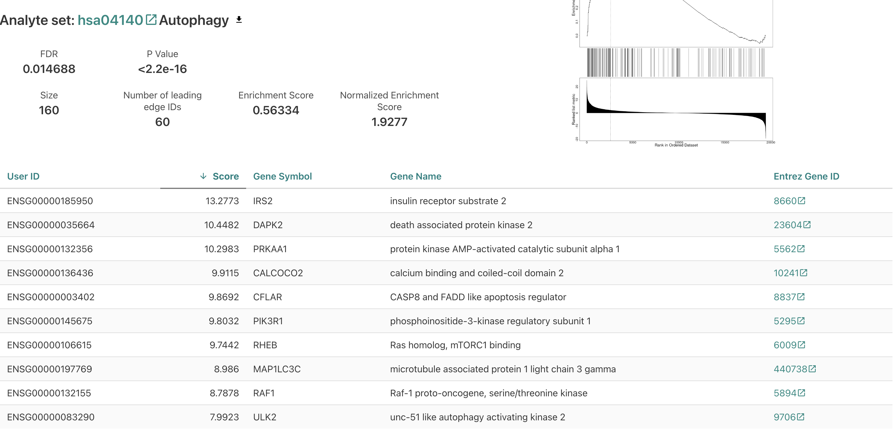
Nice! For this test we also get a value that gives the relative magnitude of change (here, all the categories seem to be ones associated with genes upregulated upon treatment).
Key Points
Normalization is necessary to account for different library sizes between samples.
Dimensional reduction (PCA) can help us understand the relationship between samples, and how it tracks with biological and technical variables.
We often want to include technical variables in the design formula, so that the differential expression comparison may include controlling for these as we solve for the effect of the biological variable.
Heatmaps are a useful visualization for understanding differential expression results, but must often be scaled by gene to become interpretable.
ORA and GSEA accept very different inputs (only DE genes versus all genes), and their outputs may be different as well as a result (though often they include similar categories).
Single-cell RNA
Overview
Teaching: 60 min
Exercises: 120 minQuestions
How can I prepare a single-cell dataset for input into analysis?
How can I evaluate the quality of a single-cell RNA-Seq dataset?
How can I visualize a single-cell dataset?
How can I annotate cell types in a single-cell dataset?
Objectives
Apply standard single-cell workflow methods such as QC filtering and normalization given a gene-cell count matrix.
Interpret the visualizations that come with a typical single-cell RNA workflow.
Implement clustering and differential expression methods to classify each cell with the proper cell type label.
Lecture portion
The workshop will include a lecture component of around one hour before the practical session later on.
Slides for this available here.
About this tutorial
This Single-cell RNA (scRNA) workflow is based on this vignette from the Satija lab, the authors of the Seurat software package.
10X Genomics (which makes a popular technology for single-cell sequencing), regularly publishes datasets to showcase the quality of their kits. This is commonly done on peripheral blood mononuclear cells (PBMCs), as these are a readily available source of human samples (blood) compared to other tissues. These samples also contain a set of easily distinguishable, well-annotated cell types (immune cells).
The 10X website provides more information and downloadable files for this dataset here.
Setting up to run this tutorial
Just as you did this morning for the bulk RNA workshop, open two tabs: one with an R notebook, and one with Terminal.
We will use the Terminal tab to download and unpack the data, and then the remainder of this workflow will be in R.
Download and unpack the data
Go to the Terminal tab.
We will be using the filtered gene-cell matrix downloaded from the following link:
https://cf.10xgenomics.com/samples/cell-exp/1.1.0/pbmc3k/pbmc3k_filtered_gene_bc_matrices.tar.gz
Download the tarball with all the files for the expression matrix using the wget command.
wget https://cf.10xgenomics.com/samples/cell-exp/1.1.0/pbmc3k/pbmc3k_filtered_gene_bc_matrices.tar.gz
List the current working directory and see the download.
ls -F
pbmc3k_filtered_gene_bc_matrices.tar.gz
Unpack the archive with tar.
tar -xvf pbmc3k_filtered_gene_bc_matrices.tar.gz
The command tar will print the path of the directories, subdirectories and files it unpacks on the screen.
filtered_gene_bc_matrices/
filtered_gene_bc_matrices/hg19/
filtered_gene_bc_matrices/hg19/matrix.mtx
filtered_gene_bc_matrices/hg19/genes.tsv
filtered_gene_bc_matrices/hg19/barcodes.tsv
Now list the current working directory.
ls -F
You should see a new directory (filtered_gene_bc_matrices/) that was not there before. List that directory (remember to try Tab to autocomplete after typing a few characters of the path).
ls -F filtered_gene_bc_matrices/
hg19/
List the sub-directory under that (remember to bring back the prior command with ↑).
ls -F filtered_gene_bc_matrices/hg19/
barcodes.tsv genes.tsv matrix.mtx
We now have the relative path to the directory with the files we need. We will use this path to load the data into R.
Single-cell workflow in R with Seurat
The following will all be run in the R notebook tab.
Load libraries.
Load all the libraries you will need for this tutorial using the library command. Today we will load Seurat, dplyr, and plyr.
library(plyr)
library(dplyr)
library(Seurat)
Read in counts and create a Seurat object.
Prepare the relative path to the directory with the files needed for the count matrix.
Based on what we saw in the data download section, what is the relative path to the directory with the files matrix.mtx, genes.tsv, and features.tsv files?
Solution
filtered_gene_bc_matrices/hg19
Read in based on the relative path.
Next, we will use the Read10X command to read in the downloaded counts, and CreateSeuratObject to create a Seurat object from this count matrix.
Let’s look at the help message for Read10X.
?Read10X
If we scroll down to the examples section, we get the following:
data_dir <- 'path/to/data/directory'
expression_matrix <- Read10X(data.dir = data_dir)
Let’s do something similar here, but replace ‘path/to/data/directory’ with the appropriate path.
Solution
data_dir = 'filtered_gene_bc_matrices/hg19'
expression_matrix = Read10X(data.dir = data_dir)
Creating the Seurat object
From the Read10X help, the next line in the example was this:
seurat_object = CreateSeuratObject(counts = expression_matrix)
If you ran the previous step as written (creating an object called expression_matrix), you should be able to run this line as-is.
Then, we can proceed with the next steps in this workflow based on our Seurat object being called seurat_object.
Quality control metrics calculation and extraction
Calculating mitochondrial rates
One important metric correlated with cell viability (dead cells have higher rates) is mitochondrial rates, or the percent of reads going to mitochondrial genes.
Here, we will use the PercentageFeatureSet argument to calculate these, and add to the Seurat object.
Generate a help message for this command.
?PercentageFeatureSetIn the example at the bottom, they run the command like so to add a variable called
percent.mtto the object, containing the mitochondrial rates.pbmc_small[["percent.mt"]] <- PercentageFeatureSet(object = pbmc_small, pattern = "^MT-")The pattern argument here means that we sum up the percent of reads going to all genes starting with
MT-, e.g.MT-ND1andMT-CO1.Let’s run this on our object, but replace
pbmc_smallwith the name of the Seurat object you just made in the previous step.Solution
seurat_object[["percent.mt"]] = PercentageFeatureSet(object = seurat_object, pattern="^MT-")QC metrics extraction
Besides the mitochondrial rates we just calculated, the following metrics are also calculated automatically when we create the Seurat object:
- nCount_RNA - Number of total UMIs per cell
- nFeature_RNA - Number of genes expressed per cell
And then based on the code we already ran, we have:
- percent.mt - Mitochondrial rate, aka % of reads in a cell that go to mitochondrial genes
We can extract these metrics from the object by using the
$operator.Let’s extract each of these metrics into a series of new objects. The example below is for
nCount_RNA. Replace the Seurat object name with the name of your object, and the name fornFeature_RNAandpercent.mtas appropriate.nCount_RNA = your_seurat_object_name$nCount_RNASolution
nCount_RNA = seurat_object$nCount_RNA
nFeature_RNA = seurat_object$nFeature_RNA
percent.mt = seurat_object$percent.mt
QC visualization
First, let’s plot a simple histogram of percent.mt, with labels.
Here is how we would make a histogram for a variable called “x”.
hist(x,label=TRUE)
Let’s do similar here, but replace percent.mt instead of x.
Solution
hist(percent.mt,label=TRUE)
It looks like there are very few cells with mitochondrial rates over 6%, and especially over 10%.
It is kind of hard to see what it is going on at the lower end of the distribution here, because the breaks in the histogram are driven by the outliers.
Let’s make another object called “percent.mt_low” that contains only the values less than 10, and then plot a histogram of that.
Example of how to subset an object by value.
x_low = x[x < 5]
We will do similar here, but with “percent.mt” instead of x and 10 instead of 5.
Solution
percent.mt_low = percent.mt[percent.mt < 10]
hist(percent.mt_low,label=TRUE)
Based on this plot, it seems like 5% would potentially be a sensible cutoff on mitochondrial rate.
But let’s make one more plot to see.
Plot nFeature_RNA vs. percent.mt. Make the point size small (cex=0.1) since we have so many points.
plot(nFeature_RNA, percent.mt, cex=0.1)
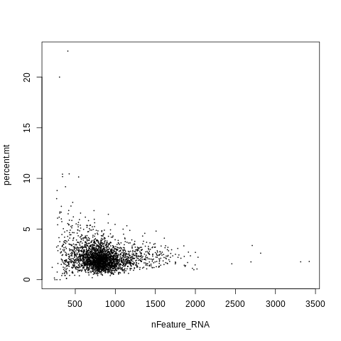
It looks like cells with mitochondrial rates over 5% tend to have very low gene counts, which is another indication of poor quality.
Let’s make a histogram of number of genes (nFeature_RNA) as well. Again, do label=TRUE.
Solution
hist(nFeature_RNA,label=TRUE)
The minimum number of genes is at least 200, which is often where people set a minimum cutoff.
On the other end of the distribution, we find that very few cells have more than 2000 genes, and the max is <= 3600.
One last plot - let’s look at the relationship between number of UMIs (nCount_RNA) and number of genes (nFeature_RNA) per cell.
plot(nCount_RNA,nFeature_RNA,cex=0.1)
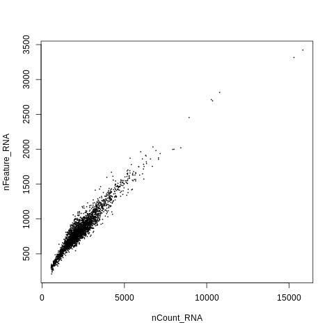
This shows a high level of linear correlation between number of UMIs and number of genes per cell, which is good! Indicates the data is high quality.
QC filtering
Based on the plots in the previous module, we are going to remove cells with mitochondrial rate less than 5% (require
percent.mt < 5).How do we do this? Let’s look up the
subsetfunction, which is a method for a Seurat object.?SeuratObject::subsetSyntax from the help message:
subset(x = seurat_object_name, subset = insert_argument_here)Example from the help message:
subset(pbmc_small, subset = MS4A1 > 4)Replace
pbmc_smallhere with the name of your Seurat object, andMS4A1 > 4with an expression to requirepercent.mtto be less than 5.your_seurat_object_name = subset(x = your_seurat_object_name, subset = your_logical_expression)Solution
seurat_object = subset(x = seurat_object, subset = percent.mt < 5)
Data normalization, variable feature selection, scaling, and dimensional reduction (PCA)
Next, we need to run the following steps:
- Normalize the data by total counts, so that cells with more coverage/RNA content can be made comparable to those with less. Also log-transform. This is done using the
NormalizeDatacommand in Seurat. - Choose a subset of genes with the most variability between cells, that we will use for downstream analysis. This is done using the
FindVariableFeaturescommand in Seurat. - Z-score (scale) the expression within each gene, for all genes in the subset from step 2. This is done using the
ScaleDatacommand in Seurat. - Run dimensional reduction (PCA) on the matrix from step 3. This is done using the
RunPCAcommand in Seurat.
Step summary
NormalizeDataFindVariableFeaturesScaleDataRunPCA
And we will just use default arguments for all of these.
Running commands on an object
This is the syntax to run a set of commands like this on an object, and add the results to the existing object:
your_object_name = command1(object=your_object_name)
your_object_name = command2(object=your_object_name)
your_object_name = command3(object=your_object_name)
your_object_name = command4(object=your_object_name)
In this lesson you will read the R package Seurat’s’ help menus and replace the example syntax above with the Seurat commands. Then replace the object name with the name of the object you have made.
Solution
seurat_object = NormalizeData(object = seurat_object)
seurat_object = FindVariableFeatures(object = seurat_object)
seurat_object = ScaleData(object = seurat_object)
seurat_object = RunPCA(object = seurat_object)
Run and plot non-linear dimensional reduction (UMAP/tSNE)
PCA can help reduce the number of dimensions that explain the data from thousands (of genes) to a handful or tens.
For visualization purposes, though, we need to be able to have a two-dimensional representation of the data.
This is where non-linear techniques like tSNE and UMAP come in. Here, we will use
UMAP, with the principal component coordinates as input.Let’s look at the help message for the command
RunUMAP.?RunUMAPScroll down to the example.
# Run UMAP map on first 5 PCs
pbmc_small <- RunUMAP(object = pbmc_small, dims = 1:5)
Main decision to make here is how many principal components to use.
In the example, they used 5. However this is very low - using the first 10 PCs is more typical for a dataset of this size.
Here, replace
pbmc_smallwith the name of your Seurat object name, and run on the first 10 PCs instead of the first 5.Solution
seurat_object = RunUMAP(object = seurat_object, dims = 1:10)There is also a command to plot the UMAP in the example.
From the example:
DimPlot(object = pbmc_small,reduction = 'umap')Replace the object name in this example with our Seurat object name, which will output a plot.
Solution
DimPlot(object = seurat_object, reduction = 'umap')
It looks like there are probably at least 3 major clusters in this data. But right now, we have not calculated those clusters yet. We will do so in the next step.
Cluster the cells
Seurat applies a graph-based clustering approach, which means that clustering requires two steps. First, we run the FindNeighbors command, which means that we calculate the distance between each cell and all other cells, and obtain the “k” nearest neighbors for each cell from these distances. Then, we use this information to obtain the clusters using the FindClusters command, where the “resolution” parameter tunes the number of clusters to be reported (higher resolution = more clusters).
Just like the UMAP command, the FindNeighbors command also works on the principal components (PCA) results.
?FindNeighbors
Scroll down to the example, where we see the following:
pbmc_small <- FindNeighbors(pbmc_small, reduction = "pca", dims = 1:10)
We want to use the first 10 PCs as input like we did for RunUMAP, so this command is almost ready to use as-is.
Just replace pbmc_small with the name of your Seurat object.
Solution
seurat_object = FindNeighbors(seurat_object,reduction = "pca", dims = 1:10)
Next, we will run the FindClusters command.
?FindClusters
From this help message, what is the default resolution for this command if you do not specify?
Solution
resolution=0.8
This seems like a good number to start with, as the Seurat documentation says that a resolution < 1 is good for a dataset with ~3000 cells.
Basic syntax of this command is similar to previous, which if we recall is:
your_object_name = yourcommand(object=your_object_name)
Run FindClusters using this syntax.
Solution
seurat_object = FindClusters(object = seurat_object)
Cluster visualization
Now, let’s run the DimPlot command again, which will now by default plot the cluster IDs on the UMAP coordinates.
DimPlot(object = seurat_object,reduction = 'umap')
It’s a bit hard to match up the colors to the legend - let’s add argument label=TRUE so we can better see what is going on.
DimPlot(object = seurat_object,reduction = 'umap',label=TRUE)

Looks like we have 11 clusters, some of which appear more distinct than others (from what we can tell from the UMAP).
Cluster annotation using canonical markers
We start with the following sets of markers.
Canonical markers of different broad PBMC cell types
CD3D: Expressed in T cells, including CD4+ and CD8+ T cellsCST3: Expressed in monocytes, dendritic cells (DCs), and plateletsGNLY: Expressed mainly in NK (natural killer) cells; can also sometimes be expressed in a subset of T cellsMS4A1: Expressed in B cellsPPBP: Expressed only in platelets
We will use these markers to annotate the clusters as one of each of the following.
Cluster labels, part 1
TMono/DC: Monocytes and dendritic cellsNKBPlatelet
Let’s make a violin plot of the expression levels of each of the marker genes.
First, pull up the help message for the violin plot command (VlnPlot).
?VlnPlot
In the example section, we find the following:
VlnPlot(object = pbmc_small, features = 'PC_1')
VlnPlot(object = pbmc_small, features = 'LYZ', split.by = 'groups')
We find that we can make a plot of either other variables like a principal component (PC_1), or expression of a gene (like LYZ).
Let’s run this command to plot the expression of the first marker, CD3D. Replace ‘pbmc_small’ with the name of our Seurat object, and ‘PC_1’ with the name of the gene of interest.
Solution
VlnPlot(object = seurat_object, features = 'CD3D')
How many clusters seem to be some kind of T cell based on this plot, and which ones?
Solution
4 clusters -
0,1,3, and5
We can add “+ NoLegend() at the end of the command, like so, to remove the legend which isn’t really necessary here.
Solution
VlnPlot(object = seurat_object, features = 'CD3D') + NoLegend()
Let’s repeat the same plotting command now, but for each of the remaining marker genes.
Then, as you generate each plot, note which clusters have high expression of the gene, and therefore which cell type they might be.
Mono/DC and platelet cluster annotation
Click the first solution below for command to plot the mono/DC marker, and a rendering of the plot.
Solution
VlnPlot(object = seurat_object, features = 'CST3') + NoLegend()
Click the second solution below for interpretation of this plot.
Solution
Clusters 4, 6, 7, 9, and 10 seem to be either mono/DC or platelets.
Click the third solution below for command to plot the platelet marker, and a rendering of the plot.
Solution
VlnPlot(object = seurat_object, features = 'PPBP') + NoLegend()
Click the fourth solution below for interpretation of this plot.
Solution
Cluster 10 seems to be platelets. Which means that clusters 4,6,7, and 9 are mono/DC.
NK and B cell cluster annotation
Plot the NK cell marker in a violin plot.
What does this tell us about which cluster(s) might be NK cells?
Solution
VlnPlot(object = seurat_object, features = 'GNLY') + NoLegend()
Clusters 3 and 8 have high expression of GNLY.
However going back to the T cell marker (CD3D) plot, cluster 3 is T cells. So, that leaves cluster 8 as NK cells.
Finally, plot the B cell marker in a violin plot, and use this to say which cluster(s) might be B cells?
Solution
VlnPlot(object = seurat_object, features = 'MS4A1') + NoLegend()
This one’s nice and straightforward! Cluster 2 is B cells, as it is the only cluster with any substantial proportion of cells expressing MS4A1.
So, to summarize, which clusters are each of the 5 broad cell types we are looking for?
Solution
T: Clusters 0,1,3,5Mono/DC: Clusters 4,6,7,9NK: Cluster 8B: Cluster 2Platelet: Cluster 10
Let’s relabel each cluster according to its broad cell types.
For broad cell types with multiple clusters, call them e.g. T_1, T_2, etc.
Relabel each cluster based on its broad cell types.
Example labels for a brain dataset:
Neuron: Clusters 0,1,5,7Astrocyte: Clusters 2,4Oligodendrocyte/OPC: Clusters 3,6Microglia: Cluster 8Code below to remap the clusters, and output a new plot with the updated cluster labels.
Note, it is important to put the cluster IDs in single quotes! Otherwise for example,
1might pull out the first level (which is cluster 0).old_cluster_ids = c('0','1','5','7','2','4','3','6','8') new_cluster_ids = c('Neuron_1','Neuron_2','Neuron_3','Neuron_4', 'Astrocyte_1','Astrocyte_2', 'Oligo/OPC_1','Oligo/OPC_2', 'Microglia') clusters = Idents(seurat_object) clusters = mapvalues(x = clusters, from = old_cluster_ids, to = new_cluster_ids) #The following is not strictly necessary, but let's also save the new cluster names as a variable called "cluster_name" in the object. seurat_object$cluster_name = clusters #Reassign the ID per cell to the cluster name instead of number. Idents(seurat_object) = clustersReplace this code with the cluster IDs and new names we just determined for this dataset (change the lines where you set
old_cluster_idsandnew_cluster_ids).Solution
old_cluster_ids = c('0','1','3','5',
  '4','6','7','9',
  '8','2','10')

new_cluster_ids = c('T_1','T_2','T_3','T_4',
  'Mono/DC_1','Mono/DC_2','Mono/DC_3','Mono/DC_4',
  'NK','B','Platelet')

clusters = Idents(seurat_object)

clusters = mapvalues(x = clusters,
  from = old_cluster_ids,
  to = new_cluster_ids)

seurat_object$cluster_name = clusters

Idents(seurat_object) = clusters
If you make a mistake and you want to reset to the old cluster IDs, here is code for how to fix it.
Then, you can re-run the code in the solution above.
Idents(seurat_object) = seurat_object$RNA_snn_res.0.8
Let’s redo the DimPlot command and see how it looks with the new, more descriptive labels.
DimPlot(object = seurat_object,reduction = 'umap',label=TRUE)
This is much improved!
Next, we are going to see if we can look at additional markers to distinguish subsets of the T cell and the Mono/DC broad cell types.
We are interested in distinguishing the following subtypes.
Cluster labels, part 2 (subtypes)
CD4+ TandCD8+ T: Two different T cell subtypesCD14+ MonocyteandFCGR3A+ Monocyte: Two different subtypes within the “Mono” subset of the “Mono/DC” clustersDendritic cell: The “DC” subset of the “Mono/DC” clusters
To distinguish these, let’s check the following markers.
Canonical markers, part 2 (subtype markers)
CD4andCD8: As the name suggests, “CD4+” T cells have high levels of CD4 protein, while “CD8+” cells have high levels of CD8 protein.FCER1A: Marker of dendritic cellsCD14andFCGR3A: Again, the proteins we expect high levels of are in the name.
We can plot two or more different genes at once in violin plot like so.
mygenes = c('Gene1','Gene2')
VlnPlot(seurat_object,features = mygenes) + NoLegend()
Let’s do this for CD4 and CD8 to start.
Distinguishing CD4+ vs. CD8+ T cell subsets
Solution
mygenes = c('CD4','CD8')
VlnPlot(seurat_object,features = mygenes) + NoLegend()
Warning message: The following requested variables were not found: CD8
Whoops! Forgot that the gene name for CD8 is actually CD8A. Just plain CD8 is the name for the protein.
Let’s try that again. Plot a violin plot of CD4 and CD8A genes.
Solution
mygenes = c('CD4','CD8A')
VlnPlot(seurat_object,features = mygenes) + NoLegend()
How do we interpret this plot?
We find that cluster T_3 seems to have high expression of CD8A.
Weirdly, none of the T cell clusters seem to have high expression of CD4.
If anything, we see a bit of expression in the Mono/DC clusters, but almost none in any of the T cell clusters.
What is going on with that?
Well, CD4 protein is expected to be high in CD4+ T cells, but not necessarily the RNA.
However, we can reasonably assume here that the T cell clusters without CD8A gene expression, are likely that way because they are CD4+ instead.
Let’s rename cluster ‘T_3’ to ‘CD8T’, and clusters ‘T_1’, ‘T_2’, and ‘T_4’ to ‘CD4T_1’, ‘CD4T_2’, and ‘CD4T_3’, the same way we renamed clusters previously.
Solution
old_cluster_ids = c('T_3','T_1','T_2','T_4')
new_cluster_ids = c('CD8T','CD4T_1','CD4T_2','CD4T_3')

clusters = Idents(seurat_object)
clusters = mapvalues(clusters,from=old_cluster_ids,to=new_cluster_ids)

Idents(seurat_object) = clusters
Let’s plot yet again.
DimPlot(object = seurat_object,reduction = 'umap',label=TRUE)
Looks great! Nice that we got the CD4 vs. CD8 T-cell annotation figured out.
Distinguishing monocyte and DC subsets
On to the remaining markers. Let’s plot FCER1A.
VlnPlot(seurat_object,features='FCER1A') + NoLegend()
And CD14 vs. FCGR3A.
mygenes = c('CD14','FCGR3A')
VlnPlot(seurat_object,features=mygenes) + NoLegend()
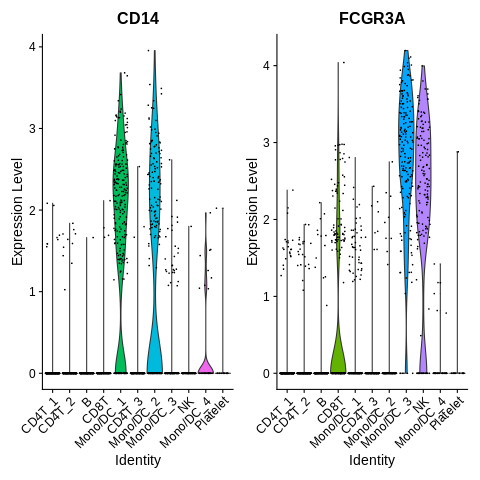
It looks like annotation should mostly be pretty straightforward here.
Except, it seems that FCGR3A is not totally just a FCGR3A+ monocyte marker, as it is also highly expressed in NK cells.
Let’s also plot another marker of FCGR3A+ monocytes, MS4A7, to make sure we are annotating correctly.
VlnPlot(seurat_object,features='MS4A7') + NoLegend()
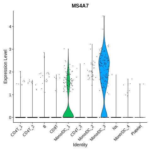
Cluster Mono/DC_3 also has high expression of this gene, in addition to the high expression of FCGR3A.
I think we are safe to label this cluster as FCGR3A+ Monocytes.
Let’s label clusters ‘Mono/DC_1’ and ‘Mono/DC_2’ as ‘CD14_Mono_1’ and ‘CD14_Mono_2’.
Cluster ‘Mono/DC_3’ as ‘FCGR3A_Mono’.
And cluster ‘Mono/DC_4’ as ‘DC’.
Solution
old_cluster_ids = c('Mono/DC_1','Mono/DC_2','Mono/DC_3','Mono/DC_4')

new_cluster_ids = c('CD14_Mono_1','CD14_Mono_2','FCGR3A_Mono','DC')

clusters = Idents(seurat_object)
clusters = mapvalues(x=clusters,from=old_cluster_ids,to=new_cluster_ids)

Idents(seurat_object) = clusters
Make UMAP plot again.
DimPlot(object = seurat_object,reduction = 'umap',label=TRUE)
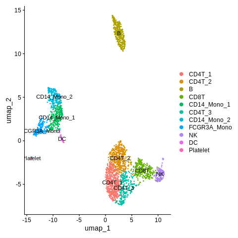
Let’s also save all these cluster names as a variable “cluster_name” within the Seurat object again.
This way, we will still have them in case we redo clustering.
seurat_object$cluster_name = Idents(seurat_object)
Re-clustering
So, the only thing about the UMAP plot above is, it seems we may have set the resolution a bit too high.
We were not expecting three different clusters of CD4+ T cells - at most we were expecting two.
Let’s try to redo the FindClusters command with a lower resolution value.
Remember, here is the command we ran previously (argument resolution=0.8 not explicitly stated previously, but it was included by default):
seurat_object = FindClusters(seurat_object,resolution=0.8)
Let’s do this again, but let’s set resolution=0.5 instead.
Solution
seurat_object = FindClusters(seurat_object,resolution=0.5)
Plot the new cluster IDs in a UMAP plot again (same command as before).
DimPlot(object = seurat_object,reduction = 'umap',label=TRUE)
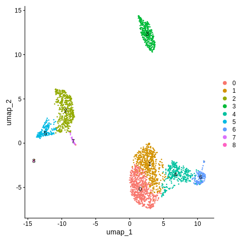
Referring back between this plot and the one before, we can re-label each of the new clusters using the same strategy we have been doing.
We now only have one cluster for CD14+ Monocytes instead of two, and two clusters for CD4+ T cells instead of three.
Solution
old_cluster_ids = c('0','1','4','6',
  '2','5','7',
  '3','8')

new_cluster_ids = c('CD4T_1','CD4T_2','CD8T','NK',
  'CD14_Mono','FCGR3A_Mono','DC',
  'B','Platelet')

clusters = Idents(seurat_object)
clusters = mapvalues(x=clusters,from=old_cluster_ids,to=new_cluster_ids)

Idents(seurat_object) = clusters
Let’s plot.
DimPlot(object = seurat_object,reduction = 'umap',label=TRUE)
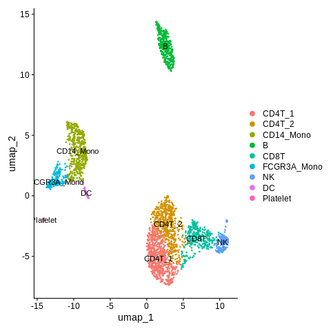
Mostly looks great! Except, I am wondering what the difference is between CD4T_1 and CD4T_2 clusters.
Let’s figure this out in the next module.
Differential expression between clusters for detailed annotation
We can use the FindMarkers command to run differential expression between groups of cells.
Let’s look at the help message for this command.
?FindMarkers
We find the following example:
markers <- FindMarkers(object = pbmc_small, ident.1 = 2)
Here, we want to run comparison between two clusters, though, so we also need to fill in the “ident.2” argument.
Here is another example from the Seurat website, where they run differential expression between cluster 5 and clusters 0 and 3 for the Seurat object “pbmc”.
cluster5.markers <- FindMarkers(pbmc, ident.1 = 5, ident.2 = c(0, 3))
Here, let’s run differential expression between CD4T_1 and CD4T_2, and save results to an object called CD4T_markers.
Remember here that our object is called seurat_object.
Solution
CD4T_markers = FindMarkers(object = seurat_object,ident.1 = 'CD4T_1',ident.2 = 'CD4T_2')
Let’s look at the first few rows.
head(CD4T_markers)
Should look something like this.
              p_val avg_log2FC pct.1 pct.2    p_val_adj
S100A4 1.119839e-77 -1.5732946 0.663 0.950 3.666129e-73
B2M    1.548560e-47 -0.3917224 1.000 1.000 5.069676e-43
IL32   2.708330e-34 -0.8913577 0.755 0.950 8.866532e-30
RPL32  1.597186e-33  0.3245829 0.998 1.000 5.228868e-29
ANXA1  2.271029e-33 -1.1805915 0.481 0.784 7.434896e-29
MALAT1 3.227506e-33  0.4359386 1.000 1.000 1.056621e-28
Here, a positive value for avg_log2FC means the gene is higher in CD4T_1 than CD4T_2.
While a negative value means the gene is higher in CD4T_2.
Let’s create two versions of this table.
One with only genes that have avg_log2FC > 0, and we’ll call it CD4T1_markers.
And the other with only genes with avg_log2FC < 0, and we’ll call it CD4T2_markers.
Solution
CD4T1_markers = CD4T_markers[CD4T_markers$avg_log2FC > 0,]
CD4T2_markers = CD4T_markers[CD4T_markers$avg_log2FC < 0,]
Next, let’s take the each of each.
head(CD4T1_markers)
              p_val avg_log2FC pct.1 pct.2    p_val_adj
RPL32  1.597186e-33  0.3245829 0.998     1 5.228868e-29
MALAT1 3.227506e-33  0.4359386 1.000     1 1.056621e-28
RPS27  3.128530e-29  0.2888005 0.998     1 1.024218e-24
RPS23  7.596983e-25  0.3204768 1.000     1 2.487100e-20
RPL21  1.258047e-24  0.3233405 0.997     1 4.118594e-20
RPS6   2.552847e-24  0.2700326 1.000     1 8.357510e-20
head(CD4T2_markers)
              p_val avg_log2FC pct.1 pct.2    p_val_adj
S100A4 1.119839e-77 -1.5732946 0.663 0.950 3.666129e-73
B2M    1.548560e-47 -0.3917224 1.000 1.000 5.069676e-43
IL32   2.708330e-34 -0.8913577 0.755 0.950 8.866532e-30
ANXA1  2.271029e-33 -1.1805915 0.481 0.784 7.434896e-29
VIM    4.209886e-32 -0.7634691 0.815 0.941 1.378232e-27
ANXA2  3.870629e-29 -1.6894050 0.158 0.468 1.267167e-24
The genes we see in the first few rows of CD4T1_markers are mostly ribosomal proteins - not the most interesting in terms of biology.
Let’s look at more rows to see if we see anything more interpretable.
head(CD4T1_markers,20)
              p_val avg_log2FC pct.1 pct.2    p_val_adj
RPL32  1.597186e-33  0.3245829 0.998 1.000 5.228868e-29
MALAT1 3.227506e-33  0.4359386 1.000 1.000 1.056621e-28
RPS27  3.128530e-29  0.2888005 0.998 1.000 1.024218e-24
RPS23  7.596983e-25  0.3204768 1.000 1.000 2.487100e-20
RPL21  1.258047e-24  0.3233405 0.997 1.000 4.118594e-20
RPS6   2.552847e-24  0.2700326 1.000 1.000 8.357510e-20
RPL9   4.138263e-23  0.3523786 0.998 0.998 1.354785e-18
RPS3A  1.893362e-20  0.3668490 0.998 1.000 6.198487e-16
RPL31  3.589483e-20  0.2982064 0.997 1.000 1.175125e-15
RPS14  7.514163e-20  0.2502883 1.000 1.000 2.459987e-15
CCR7   7.396108e-19  1.2961428 0.467 0.246 2.421338e-14
RPS13  8.350707e-19  0.2985510 0.989 0.987 2.733855e-14
RPL13  1.203840e-18  0.2420806 1.000 1.000 3.941133e-14
RPL11  5.276883e-15  0.2304492 1.000 1.000 1.727546e-10
RPL30  7.408685e-15  0.2386593 1.000 1.000 2.425455e-10
RPS28  1.996393e-14  0.2641382 0.992 0.992 6.535791e-10
RPS16  2.500937e-14  0.2595951 0.997 0.998 8.187568e-10
RPLP2  3.838422e-14  0.2096304 1.000 1.000 1.256623e-09
RPL19  1.000814e-13  0.1726900 0.998 1.000 3.276464e-09
RPS25  1.027298e-13  0.2320915 0.998 0.998 3.363167e-09
We find a gene called CCR7 is upregulated in CD4T_1.
Let’s say we didn’t know a lot about the biology here. Maybe we can Google it and see what comes up?
One solution below - but you may word your search differently!
Solution
We also find that a gene called S100A4 is the top most significantly upregulated gene in CD4T_2.
Let’s try a search again. One possibly search query below.
Solution
Well, that is not the most helpful. Seems like both of these genes can be expressed in memory CD4+ T cells?
What if we edit the search to specifically focus on CD4+ T cells, not just all T cells? Maybe that will help?
Solution
OK, so it looks like Ccr7 can be expressed in either naive CD4+ T cells, or specifically central memory T cells.
While effector memory T cells do not express this gene.
This also makes sense with what we saw when we searched for S100A4, which is expressed specifically in effector memory T cells.
If we search for more info on naive vs. memory T cells, we also find this paper, which seems to confirm the initial Google AI overview, so we aren’t just relying on that.
Let’s annotate these clusters based on this (CD4T_1 = Naive_or_central_memory_CD4T, CD4T_2 = Effector_memory_CD4T), but put a “?” since it’s a bit iffy compared to the other cluster annotation.
In a real-world analysis, this would often be the time to do a deeper literature review, or consult a collaborator with more knowledge of the biology to confirm this preliminary annotation.
old_cluster_ids = c('CD4T_1','CD4T_2')
new_cluster_ids = c('Naive_or_central_memory_CD4T?','Effector_memory_CD4T?')

clusters = Idents(seurat_object)
clusters = mapvalues(x=clusters,from=old_cluster_ids,to=new_cluster_ids)

Idents(seurat_object) = clusters
Final plot:
DimPlot(object = seurat_object,reduction = 'umap',label=TRUE)
Also think we can remove the legend here.
DimPlot(object = seurat_object,reduction = 'umap',label=TRUE) + NoLegend()
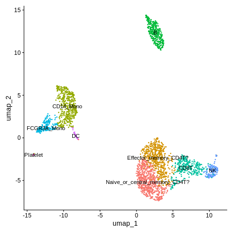
Key Points
Single-cell RNA analysis often starts with a gene-cell count matrix.
QC metrics used for understanding and filtering data quality include mitochondrial rate and number of genes.
Processing stages in a scRNA workflow includes normalization, feature selection, scaling, and dimensional reduction.
Clustering is a key step in understanding biology.
We can use known marker genes or run differential expression between clusters to annotate cell types after clustering.
Annotation often requires starting with broad cell types, then moving to more specific.


