Overview

Teaching: 60 min
Exercises: 120 min

Questions

• How do I normalize a bulk RNA dataset?

• How can I summarize the relationship between samples?

• How can I compare expression based on biological or technical variables?

• How can I visualize the results of this comparison?

• How can I prepare differential expression results for input into downstream tools for biological insight?

• How can I interpret the results of functional enrichment tools?

Objectives

• Apply standard bulk workflow pre-processing methods such as DESeq2 normalization given a gene-sample count matrix.

• Execute dimensional reduction (PCA) and corresponding visualization.

• Understand design formulas and how to apply them to run differential expression.

• Summarize differential expression (DE) results using a heatmap visualization as well as MA and volcano plots.

• Interpret data visualizations from the above steps.

• Use base R commands to output text files from DE results for input into functional enrichment (ORA/GSEA).

• Run ORA/GSEA using a web-based tool, and describe the meaning of the resulting output.

Lecture portion

The workshop will include a lecture component of around one hour before the practical session later on.

Slides for this available here.

About this tutorial

This workflow is based on material from the rnaseqGene page on Bioconductor (link).

This data is from a published dataset of an RNA-Seq experiment on airway smooth muscle (ASM) cell lines. From the abstract:

“Using RNA-Seq, a high-throughput sequencing method, we characterized transcriptomic changes in four primary human ASM cell lines that were treated with dexamethasone - a potent synthetic glucocorticoid (1 micromolar for 18 hours).”

Citation:

Himes BE, Jiang X, Wagner P, Hu R, Wang Q, Klanderman B, Whitaker RM, Duan Q, Lasky-Su J, Nikolos C, Jester W, Johnson M, Panettieri R Jr, Tantisira KG, Weiss ST, Lu Q. “RNA-Seq Transcriptome Profiling Identifies CRISPLD2 as a Glucocorticoid Responsive Gene that Modulates Cytokine Function in Airway Smooth Muscle Cells.” PLoS One. 2014 Jun 13;9(6):e99625. PMID: 24926665. GEO: GSE52778

DOI link here.

Setting up to run this tutorial

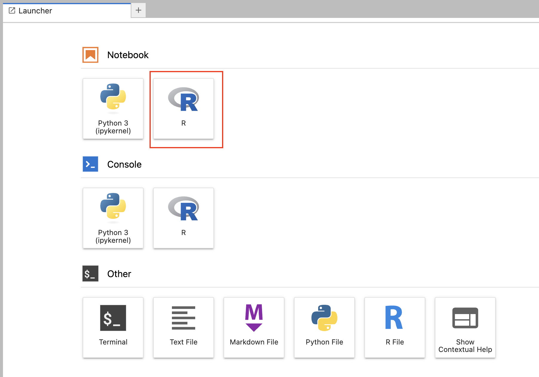
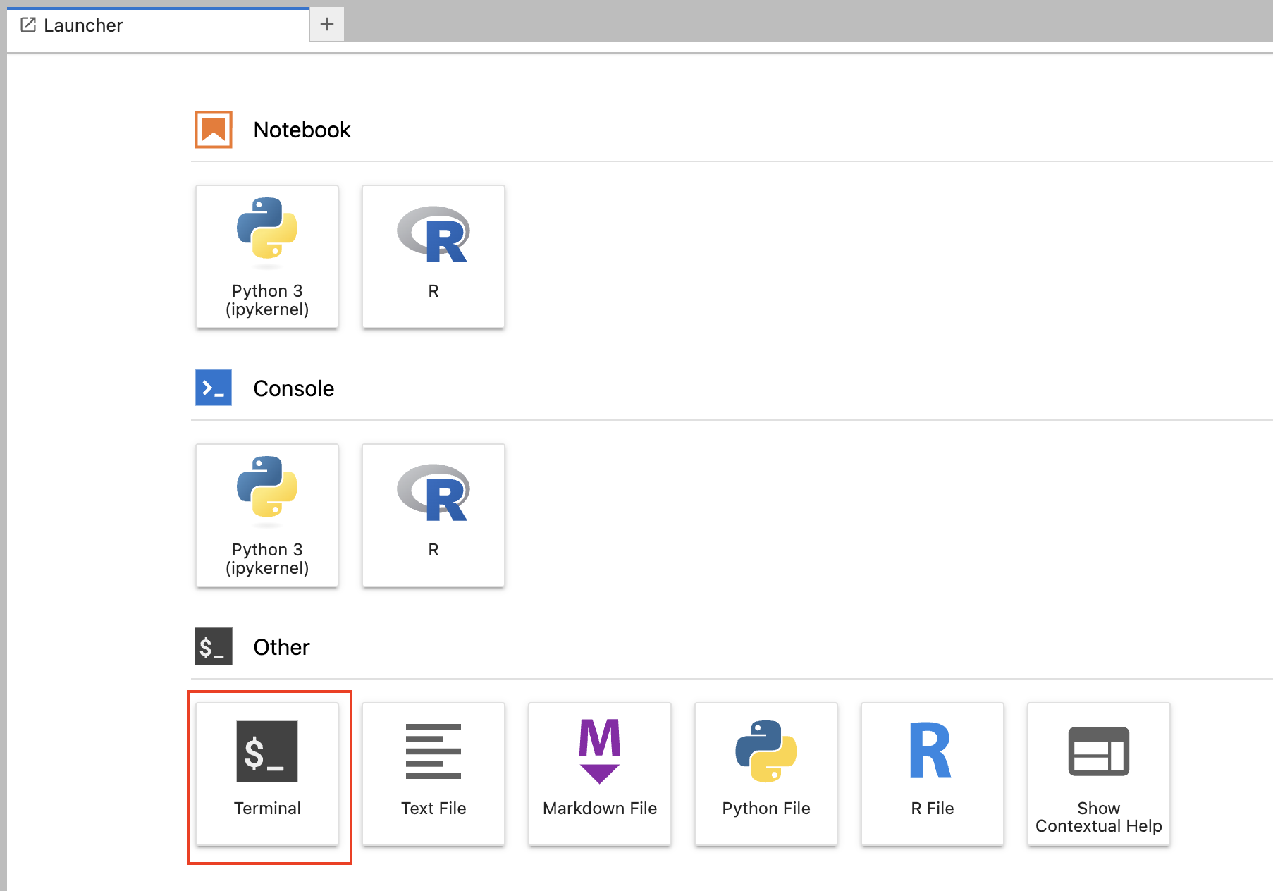
Open Launcher.

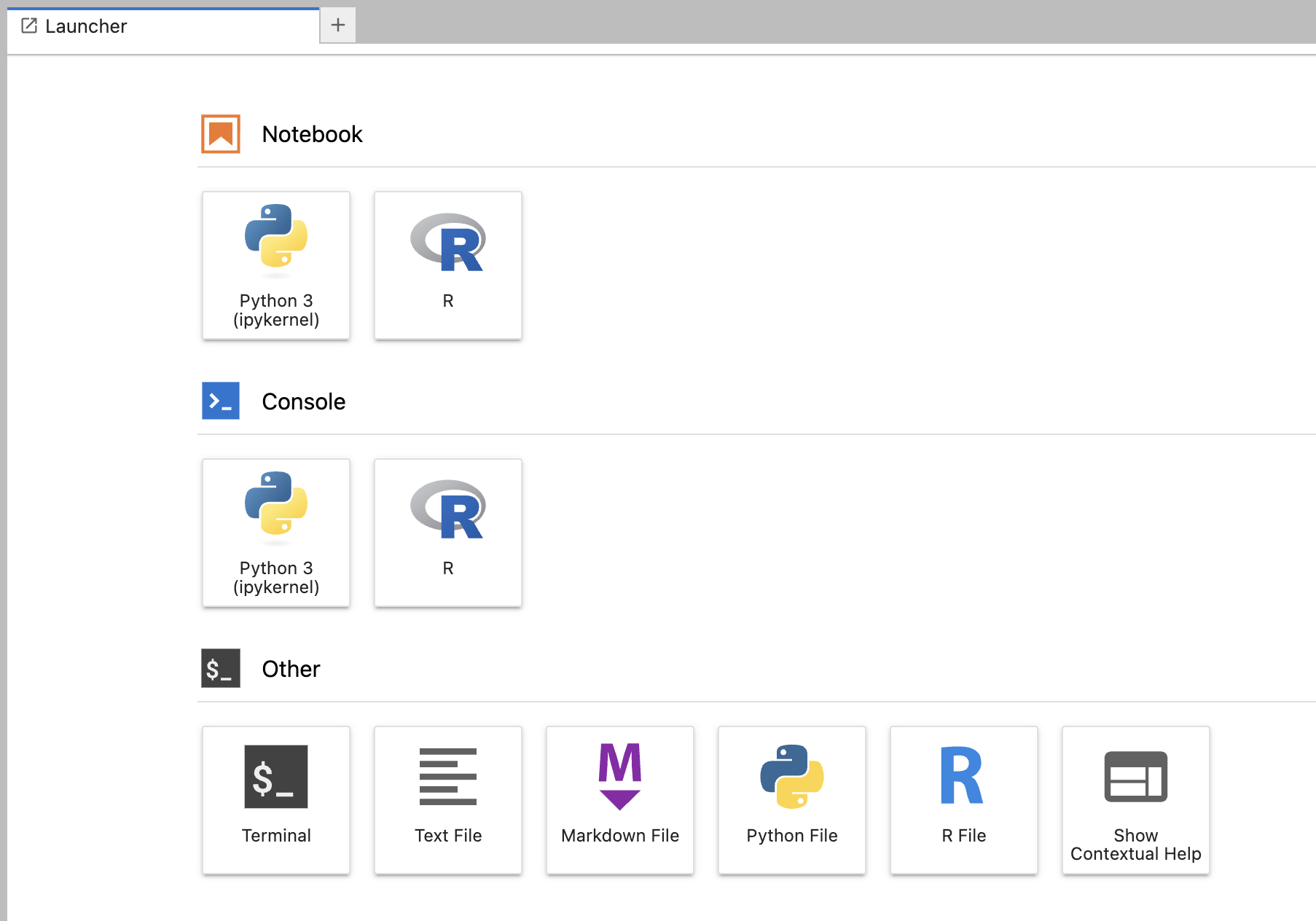
Go to “R” under “Notebook”.

Press the “+” at the top to open another tab.

This time, go to “Other”, then “Terminal”.

Locating the data on the file system

This section will be run in the “Terminal” tab.

The data has already been downloaded, and is in CSV format for easy reading into R.

The main files we will be working with today are a gene x sample count matrix, and a metadata file with design information for the samples.

Data is available in this directory:

/data/RNA/bulk

If we list that path like so:

ls /data/RNA/bulk

We find the following files:

airway_raw_counts.csv.gz
airway_sample_metadata.csv

To list the files with their full paths, we can use *.

ls /data/RNA/bulk/*

/data/RNA/bulk/airway_raw_counts.csv.gz  /data/RNA/bulk/airway_sample_metadata.csv

Bulk RNA differential expression workflow in R with DESeq2

The following will all be run in the R notebook tab.

However, let’s also leave the Terminal tab open for later.

Load libraries.

Load all the libraries you will need for this tutorial using the library command. Today we will load DESeq2, ggplot2, and pheatmap.

library(DESeq2)
library(ggplot2)
library(pheatmap)

Reading in files and basic data exploration.

First, before we read anything into R, what is the full path to the raw counts file?

Solution

/data/RNA/bulk/airway_raw_counts.csv.gz

Use this to read into R using the read.csv command.

Let’s read the help message for this command.

?read.csv

Main argument here is file. Let’s try filling in the path from above.

Solution

read.csv(file=/data/RNA/bulk/airway_raw_counts.csv.gz)

Error in parse(text = x, srcfile = src): <text>:1:15: unexpected '/'
1: read.csv(file=/
^Traceback:

Oops, let’s fix that.

Solution

read.csv(file="/data/RNA/bulk/airway_raw_counts.csv.gz")

A data.frame: 63677 × 9
gene_id	SRR1039508	SRR1039509	SRR1039512	SRR1039513	SRR1039516	SRR1039517	SRR1039520	SRR1039521
<chr>	<int>	<int>	<int>	<int>	<int>	<int>	<int>	<int>
ENSG00000000003	679	448	873	408	1138	1047	770	572
ENSG00000000005	0	0	0	0	0	0	0	0
ENSG00000000419	467	515	621	365	587	799	417	508
ENSG00000000457	260	211	263	164	245	331	233	229
ENSG00000000460	60	55	40	35	78	63	76	60
ENSG00000000938	0	0	2	0	1	0	0	0
ENSG00000000971	3251	3679	6177	4252	6721	11027	5176	7995
ENSG00000001036	1433	1062	1733	881	1424	1439	1359	1109
ENSG00000001084	519	380	595	493	820	714	696	704
ENSG00000001167	394	236	464	175	658	584	360	269
...
ENSG00000273484	0	0	0	0	0	0	0	0
ENSG00000273485	2	3	1	1	1	1	1	0
ENSG00000273486	14	11	25	8	20	32	12	11
ENSG00000273487	5	9	4	11	10	10	4	10
ENSG00000273488	7	5	8	3	8	16	11	14
ENSG00000273489	0	0	0	1	0	1	0	0
ENSG00000273490	0	0	0	0	0	0	0	0
ENSG00000273491	0	0	0	0	0	0	0	0
ENSG00000273492	0	0	1	0	0	0	0	0
ENSG00000273493	0	0	0	0	1	0	0	0

Looks like we just read in as standard input/output, rather than saving to an object.

Let’s save the result of this command in an object called raw.counts.

Solution

raw.counts = read.csv(file="/data/RNA/bulk/airway_raw_counts.csv.gz")

Use the head command to look at the first few lines.

head(raw.counts)

          gene_id SRR1039508 SRR1039509 SRR1039512 SRR1039513 SRR1039516
1 ENSG00000000003        679        448        873        408       1138
2 ENSG00000000005          0          0          0          0          0
3 ENSG00000000419        467        515        621        365        587
4 ENSG00000000457        260        211        263        164        245
5 ENSG00000000460         60         55         40         35         78
6 ENSG00000000938          0          0          2          0          1
  SRR1039517 SRR1039520 SRR1039521
1       1047        770        572
2          0          0          0
3        799        417        508
4        331        233        229
5         63         76         60
6          0          0          0

Looks like the first column is the gene ids.

It would be better if we could read in such that it would automatically make those the row names, so that all the values in the table could be numeric.

Let’s look at the read.csv help message again to see if there is a way to do that.

?read.csv

If we scroll down we find the following:

row.names: a vector of row names.  This can be a vector giving the
          actual row names, or a single number giving the column of the
          table which contains the row names, or character string
          giving the name of the table column containing the row names.

Let’s use this argument to read in the file again using read.csv, this time taking the first column as the row names.

Solution

raw.counts = read.csv(file="/data/RNA/bulk/airway_raw_counts.csv.gz",row.names=1)

Look at the first few lines of raw.counts again.

head(raw.counts)

                SRR1039508 SRR1039509 SRR1039512 SRR1039513 SRR1039516
ENSG00000000003        679        448        873        408       1138
ENSG00000000005          0          0          0          0          0
ENSG00000000419        467        515        621        365        587
ENSG00000000457        260        211        263        164        245
ENSG00000000460         60         55         40         35         78
ENSG00000000938          0          0          2          0          1
                SRR1039517 SRR1039520 SRR1039521
ENSG00000000003       1047        770        572
ENSG00000000005          0          0          0
ENSG00000000419        799        417        508
ENSG00000000457        331        233        229
ENSG00000000460         63         76         60
ENSG00000000938          0          0          0

Looks good! Think we are ready to proceed with this object now.

Check how many rows there are.

nrow(raw.counts)

[1] 63677

So, we have 63,677 genes, and 8 samples (as we saw when we did head).

Next, read in the file with the study design.

Remember path to this file is:

/data/RNA/bulk/airway_sample_metadata.csv

We can once again use the csv command, and take the first column as row names.

Read into an object called expdesign.

Solution

expdesign = read.csv(file="/data/RNA/bulk/airway_sample_metadata.csv",row.names=1)

Look at the object.

expdesign

              cell   dex avgLength
SRR1039508  N61311 untrt       126
SRR1039509  N61311   trt       126
SRR1039512 N052611 untrt       126
SRR1039513 N052611   trt        87
SRR1039516 N080611 untrt       120
SRR1039517 N080611   trt       126
SRR1039520 N061011 untrt       101
SRR1039521 N061011   trt        98

We are mainly interested in columns cell (says which of the four cell lines the sample is) and dex (says whether or not the sample had drug treatment) here.

Making a DESeq object using DESeq2

We are going to take the raw counts matrix, and the experimental design matrix, and make a special type of object called a DESeqDataSet.

We are going to use a function DESeqDataSetFromMatrix, from the DESeq2 library that we already loaded, to do this.

Let’s view the help message for that function.

?DESeqDataSetFromMatrix

Start of the help message looks like this:

DESeqDataSetFromMatrix(
       countData,
       colData,
       design,
       tidy = FALSE,
       ignoreRank = FALSE,
       ...
     )

We also find the following if we scroll down to the example:

countData <- matrix(1:100,ncol=4)
condition <- factor(c("A","A","B","B"))
dds <- DESeqDataSetFromMatrix(countData, DataFrame(condition), ~ condition)

If we explicitly stated the arguments in the example (and named the objects less confusingly), it would look like this:

mycounts = matrix(1:100,ncol=4)
group = factor(c("A","A","B","B"))
expdesign_example = data.frame(condition = group)
#expdesign_example now looks like this:
#  condition
#1         A
#2         A
#3         B
#4         B
dds = DESeqDataSetFromMatrix(countData = mycounts,
  colData = expdesign_example,
  design = ~condition)

Let’s run this for our data set, but using raw.counts as the count matrix and expdesign as the design matrix.

For the design, let’s look at the column names of expdesign again.

colnames(expdesign)

[1] "cell"      "dex"       "avgLength"

Here, we want to include both the cell line (cell) and treatment status (dex) in the design.

Save to an object called myDESeqObject.

Solution

myDESeqObject = DESeqDataSetFromMatrix(countData = raw.counts,
  colData = expdesign,
  design = cell,dex)

Error: object 'dex' not found

Oops, looks like we did something wrong.

Should we be putting cell and dex in quotes maybe? That worked the last time we got this kind of error.

Solution

myDESeqObject = DESeqDataSetFromMatrix(countData = raw.counts,
  colData = expdesign,
  design = c("cell","dex"))

Error in DESeqDataSet(se, design = design, ignoreRank) : 
'design' should be a formula or a matrix

Hm, still not right.

I think what we are looking for is a design formula here.

If you search for how to make a design formula, you can find this guide, where we seem to see the following rules:

• Design formula should always start with ~.
• If more than one variable, put a + in between.
• Nothing in quotes.

For example, their formula for the variables diet and sex was this:

~diet + sex

Let’s see if we can finally fix our command to properly set the design to include cell and dex here.

Solution

myDESeqObject = DESeqDataSetFromMatrix(countData = raw.counts,
  colData = expdesign,
  design = ~cell + dex)

When we run the above, we get the following output:

Warning message:
In DESeqDataSet(se, design = design, ignoreRank) :
some variables in design formula are characters, converting to factors

This is just a warning message, doesn’t mean we did anything wrong.

Looks like the command finally ran OK!

Normalization on the DESeq object

We will next run the estimateSizeFactors command on this object, and save the output back to myDESeqObject.

This command prepares the object for the next step, where we normalize the data by library size (total counts).

myDESeqObject = estimateSizeFactors(myDESeqObject)

Next, we will run a normalization method called rlogTransformation (regularized-log transformation) on myDESeqObject, and save to a new object called rlogObject.

Basic syntax for how this works:

transformedObject = transformationCommand(object = oldObject)

Replace transformedObject here with the name we want for the new object, and transformationCommand with rlogTransformation. Here the oldObject is the DESeq object we already made.

Solution

rlogObject = rlogTransformation(object = myDESeqObject)

Let’s also save just the normalized values from rlogObject in a separate object called rlogMatrix.

rlogMatrix = assay(rlogObject)

Principal components analysis (PCA)

We will run DESeq2’s plotPCA function on the object produced by the rlogTransformation command, to create a plot where we can see the relationship between samples by reducing into two dimensions.

Again, let’s view the help message for this function.

?plotPCA

We find the following documentation.

Usage:

     ## S4 method for signature 'DESeqTransform'
     plotPCA(object, intgroup = "condition", ntop = 500, returnData = FALSE)
     
Arguments:

  object: a ‘DESeqTransform’ object, with data in ‘assay(x)’, produced
          for example by either ‘rlog’ or
          ‘varianceStabilizingTransformation’.

intgroup: interesting groups: a character vector of names in
          ‘colData(x)’ to use for grouping

Examples:

dds <- makeExampleDESeqDataSet(betaSD=1)
vsd <- vst(dds, nsub=500)
plotPCA(vsd)

A more explicitly stated version of the example:

dds = makeExampleDESeqDataSet(betaSD=1)
raw.counts_example = assay(dds)
expdesign_example = colData(dds)
head(raw.counts_example)
expdesign_example

sample1	sample2	sample3	sample4	sample5	sample6	sample7	sample8	sample9	sample10	sample11	sample12
gene1	6	6	2	8	17	2	0	4	17	7	3	10
gene2	27	48	40	26	12	39	7	5	4	14	9	6
gene3	8	7	4	2	1	1	2	21	4	2	9	0
gene4	36	24	41	25	44	25	39	19	8	31	17	62
gene5	22	36	10	28	33	9	55	58	71	12	68	22
gene6	1	12	5	6	15	1	2	0	7	4	0	1

DataFrame with 12 rows and 1 column
         condition
          <factor>
sample1          A
sample2          A
sample3          A
sample4          A
sample5          A
...            ...
sample8          B
sample9          B
sample10         B
sample11         B
sample12         B

dds = DESeqDataSetFromMatrix(countData = raw.counts_example,
    colData = expdesign_example,
    design=~condition)
vsd <- vst(dds, nsub=500)
plotPCA(object = vsd)

We already ran DESeqDataSetFromMatrix, as well as transformation (we ran rlogTransformation instead of vst, but same idea).

So, just need to plug the object from rlogTransformation into plotPCA.

Solution

plotPCA(object = rlogObject)

Error in .local(object, ...) : 
the argument 'intgroup' should specify columns of colData(dds)

In the example, we did not need to explicitly state what variable to color by in the plot, since there was only one (condition).

However here, we have two possible variables , so we need to explicitly state.

In the example, if we had explicitly stated to color by condition, it would look like this.

plotPCA(object = vsd, intgroup = "condition")

Let’s use the same syntax here to try running plotPCA on rlogObject again, this time explicitly stating to color by cell using the intgroup argument.

Solution

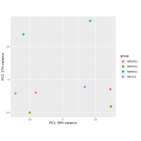
plotPCA(object = rlogObject, intgroup = "cell")

Next, repeat but this time color by dex.

Solution

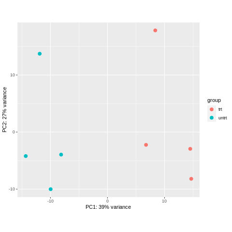
plotPCA(object = rlogObject, intgroup = "dex")

Interpreting the PCA plot

Let’s look at the two plots we made, and answer the following.

• What principal component separates the four different cell lines? Which one separates treated vs. untreated?
• How much variance is explained by each principal component (hint: see axis labels)?

Solution

PC2 separates the four different cell lines. PC1 separates treated vs. untreated.

PC1 explains 39% of the variance. PC2 explains 27% of the variance.

Differential expression testing

Now that we have created the DESeq object, and done some initial data exploration, it is time to run differential expression testing to see which genes are significantly different between conditions (here, drug-treated vs. not drug-treated).

One step we need to run to get these results is the command DESeq. Let’s pull up the help message for this.

?DESeq

Start of this help message:

Usage:

     DESeq(
       object,
       test = c("Wald", "LRT"),
       fitType = c("parametric", "local", "mean", "glmGamPoi"),
       sfType = c("ratio", "poscounts", "iterate"),
       betaPrior,
       full = design(object),
       reduced,
       quiet = FALSE,
       minReplicatesForReplace = 7,
       modelMatrixType,
       useT = FALSE,
       minmu = if (fitType == "glmGamPoi") 1e-06 else 0.5,
       parallel = FALSE,
       BPPARAM = bpparam()
     )
     
Arguments:

  object: a DESeqDataSet object, see the constructor functions
          ‘DESeqDataSet’, ‘DESeqDataSetFromMatrix’,
          ‘DESeqDataSetFromHTSeqCount’.

Seems like we can just input our DESeqDataSet object to the object argument?

Let’s do that, and save as a new object called dds.

dds = DESeq(object = myDESeqObject)

If all goes well, you should get the following output as the command runs.

using pre-existing size factors
estimating dispersions
gene-wise dispersion estimates
mean-dispersion relationship
final dispersion estimates
fitting model and testing

Next, we will need to run the results function on dds.

Now, pull up the help message for that function.

?results

Usage:

     results(
       object,
       contrast,
       name,
       lfcThreshold = 0,
...)

Arguments:

  object: a DESeqDataSet, on which one of the following functions has
          already been called: ‘DESeq’, ‘nbinomWaldTest’, or
          ‘nbinomLRT’

contrast: this argument specifies what comparison to extract from the
          ‘object’ to build a results table. one of either:

            • a character vector with exactly three elements: the name
              of a factor in the design formula, the name of the
              numerator level for the fold change, and the name of the
              denominator level for the fold change (simplest case)

...

Examples:

     ## Example 1: two-group comparison
     
     dds <- makeExampleDESeqDataSet(m=4)
     
     dds <- DESeq(dds)
     res <- results(dds, contrast=c("condition","B","A"))

To highlight the example:

dds <- DESeq(dds)
res <- results(dds, contrast=c("condition","B","A"))

Replace condition, B, and A with the appropriate values for this data set.

We are looking to compare the effect of treatment with the drug.

Let’s look at our experimental design matrix again.

expdesign

              cell   dex avgLength
SRR1039508  N61311 untrt       126
SRR1039509  N61311   trt       126
SRR1039512 N052611 untrt       126
SRR1039513 N052611   trt        87
SRR1039516 N080611 untrt       120
SRR1039517 N080611   trt       126
SRR1039520 N061011 untrt       101
SRR1039521 N061011   trt        98

Filling in the contrast argument to results from expdesign

Some questions we need to answer here are:

• What is the variable name for drug treatment here?
• What are the two levels of this variable?
• What order should we put these two levels in, if we want untreated to be the baseline?

Solution

• The variable name for drug treatment is dex.
• The two levels are trt and untrt.
• We should put trt first and untrt second so that the fold-change will be expressed as treated/untreated.

Now that we figured that out, we just need to plug everything into the function.

Output to an object called res.

Solution

res = results(object = dds, contrast = c("dex","trt","untrt"))

Let’s look at the first few rows of the results using head.

head(res)

log2 fold change (MLE): dex trt vs untrt 
Wald test p-value: dex trt vs untrt 
DataFrame with 6 rows and 6 columns
                  baseMean log2FoldChange     lfcSE      stat      pvalue
                 <numeric>      <numeric> <numeric> <numeric>   <numeric>
ENSG00000000003 708.602170     -0.3812540  0.100654 -3.787752 0.000152016
ENSG00000000005   0.000000             NA        NA        NA          NA
ENSG00000000419 520.297901      0.2068126  0.112219  1.842943 0.065337292
ENSG00000000457 237.163037      0.0379204  0.143445  0.264356 0.791505742
ENSG00000000460  57.932633     -0.0881682  0.287142 -0.307054 0.758801924
ENSG00000000938   0.318098     -1.3782270  3.499873 -0.393793 0.693733530
                      padj
                 <numeric>
ENSG00000000003 0.00128292
ENSG00000000005         NA
ENSG00000000419 0.19646985
ENSG00000000457 0.91141962
ENSG00000000460 0.89500478
ENSG00000000938         NA

Run the following to get an explanation of what each column in this output means.

mcols(res)$description

[1] "mean of normalized counts for all samples"
[2] "log2 fold change (MLE): dex trt vs untrt" 
[3] "standard error: dex trt vs untrt"         
[4] "Wald statistic: dex trt vs untrt"         
[5] "Wald test p-value: dex trt vs untrt"      
[6] "BH adjusted p-values"

Ready to start to explore and interpret these results.

Visualizing expression of differentially expressed genes (heatmap)

Use the which function to get the indices (row numbers) of the genes with adjusted p-value < .01 (false discovery rate of 1%).

Then, save as an object called degs.

First, which column index or name contains the adjusted p-values?

Solution

Column "padj", or column number 6.

Then, we will need to extract this column. A few possible ways listed below.

Solution

res$padj
res[,6]
res[,"padj"]

Next, help message for the which command (from base package) gives the following:

Usage:

     which(x, arr.ind = FALSE, useNames = TRUE)
     arrayInd(ind, .dim, .dimnames = NULL, useNames = FALSE)
     
Arguments:

       x: a ‘logical’ vector or array.  ‘NA’s are allowed and omitted
          (treated as if ‘FALSE’).

Examples:

     which(LETTERS == "R")
..
which(1:10 > 3, arr.ind = TRUE)

So, we just need to add a statement to get only values less than 0.01 from the column.

Solution

degs = which(res$padj < .01)

How many differentially expressed genes do we find?

length(degs)

[1] 2901

Next, let’s subset the normalized expression matrix (rlogMatrix) to only these genes, and output to a new matrix rlogMatrix.degs.

Syntax of matrix subsetting:

mydat.subset = mydat[indices_to_subset,]

Solution

rlogMatrix.degs = rlogMatrix[degs,]

Let’s run the pheatmap command on this matrix to output a heatmap to the console.

pheatmap(object = rlogMatrix.degs)

Error in pheatmap(object = rlogMatrix.degs) : 
  argument "mat" is missing, with no default

Well, that’s why we should read the help message! Seems the main argument for the input object to pheatmap is mat, not object.

pheatmap(mat = rlogMatrix.degs)

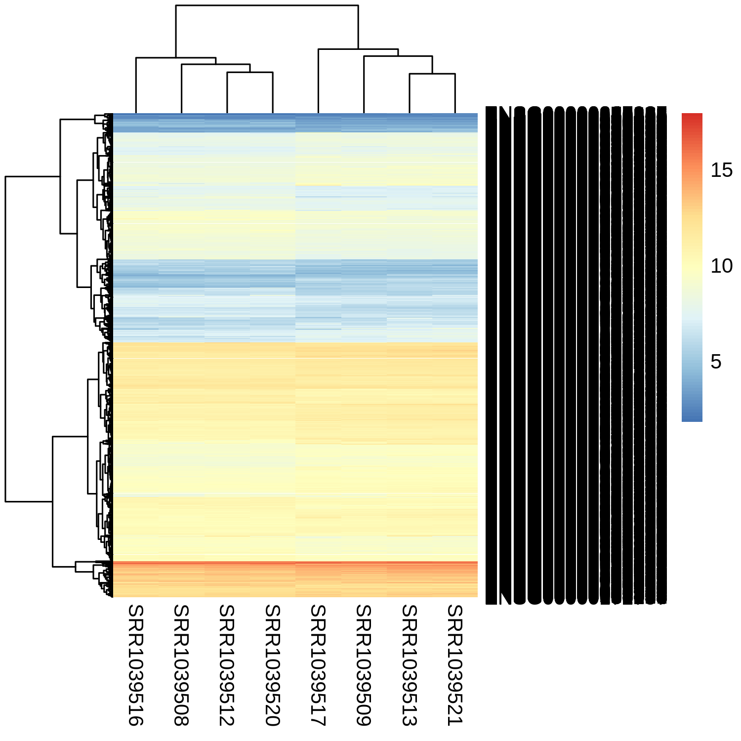
Does not seem super informative!

Let’s look at the pheatmap help message again and see if we can add some arguments to make it better.

?pheatmap

Scrolling down to arguments, we see:

scale: character indicating if the values should be centered and
          scaled in either the row direction or the column direction,
          or none. Corresponding values are ‘"row"’, ‘"column"’ and
          ‘"none"’

Let’s scale across the genes, so by row.

And also this:

show_rownames: boolean specifying if row names are be shown.

Boolean means either TRUE or FALSE. Let’s turn this off.

Solution

pheatmap(mat = rlogMatrix.degs,
    scale="row",
    show_rownames=FALSE)

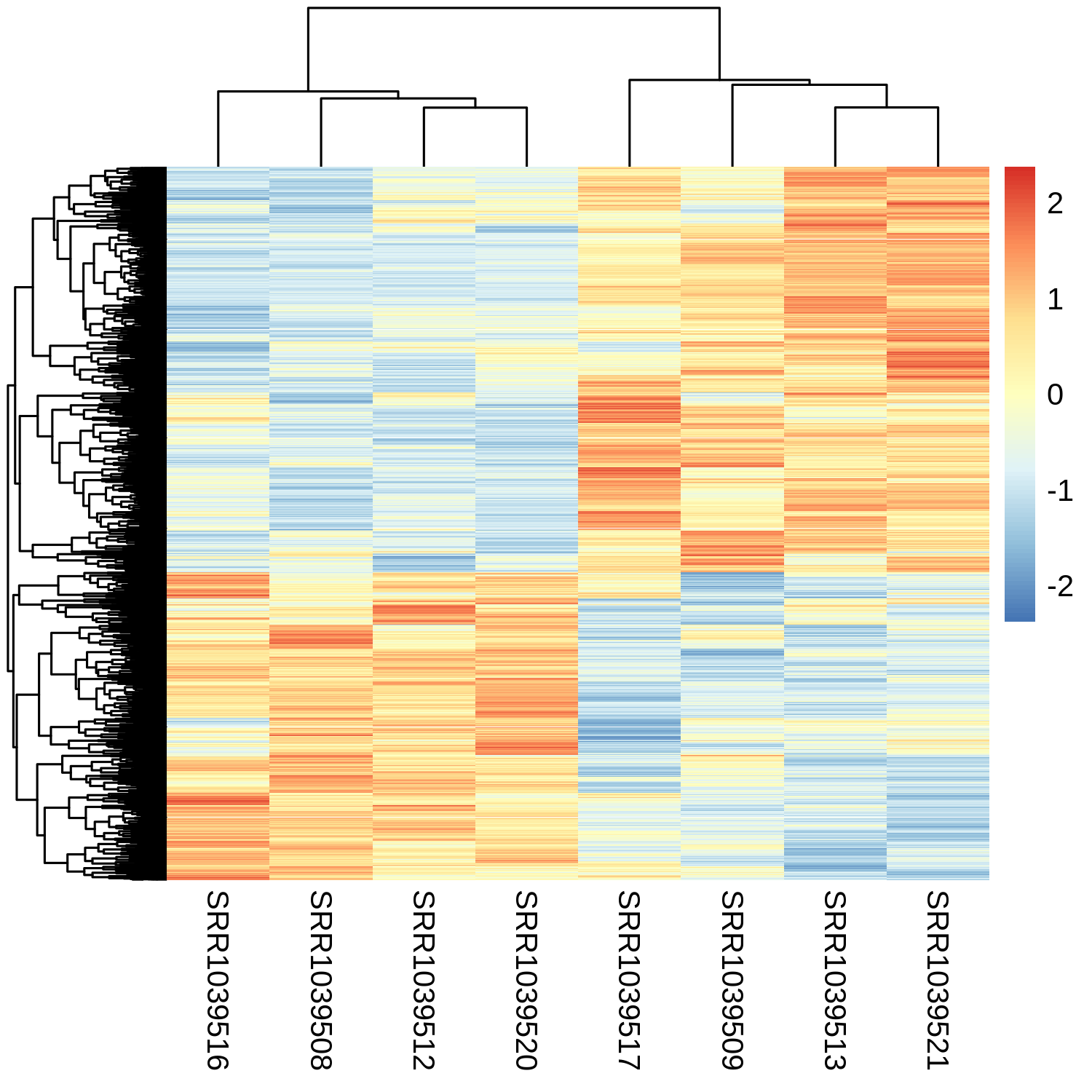
Think we mostly have what we want now.

Except, the “SRR” sample names are not very informative.

It would be good to have an annotation bar at the top of the heatmap that said what cell line each sample is from, and whether it is treated or untreated.

Going back to the pheatmap help message:

annotation_row: data frame that specifies the annotations shown on left
          side of the heatmap. Each row defines the features for a
          specific row. The rows in the data and in the annotation are
          matched using corresponding row names. Note that color
          schemes takes into account if variable is continuous or
          discrete.

annotation_col: similar to annotation_row, but for columns.

We already have a data frame with the annotation we are looking for, so just need to give it as an argument here.

Solution

pheatmap(mat = rlogMatrix.degs,
    scale="row",
    show_rownames=FALSE,
    annotation_row=expdesign)

Error in seq.int(rx[1L], rx[2L], length.out = nb) : 
'from' must be a finite number
In addition: Warning messages:
1: In min(x) : no non-missing arguments to min; returning Inf
2: In max(x) : no non-missing arguments to max; returning -Inf

Oops - looks like we used the wrong argument. We want to annotate the samples, not the genes.

Solution

pheatmap(mat = rlogMatrix.degs,
    scale="row",
    show_rownames=FALSE,
    annotation_col=expdesign)

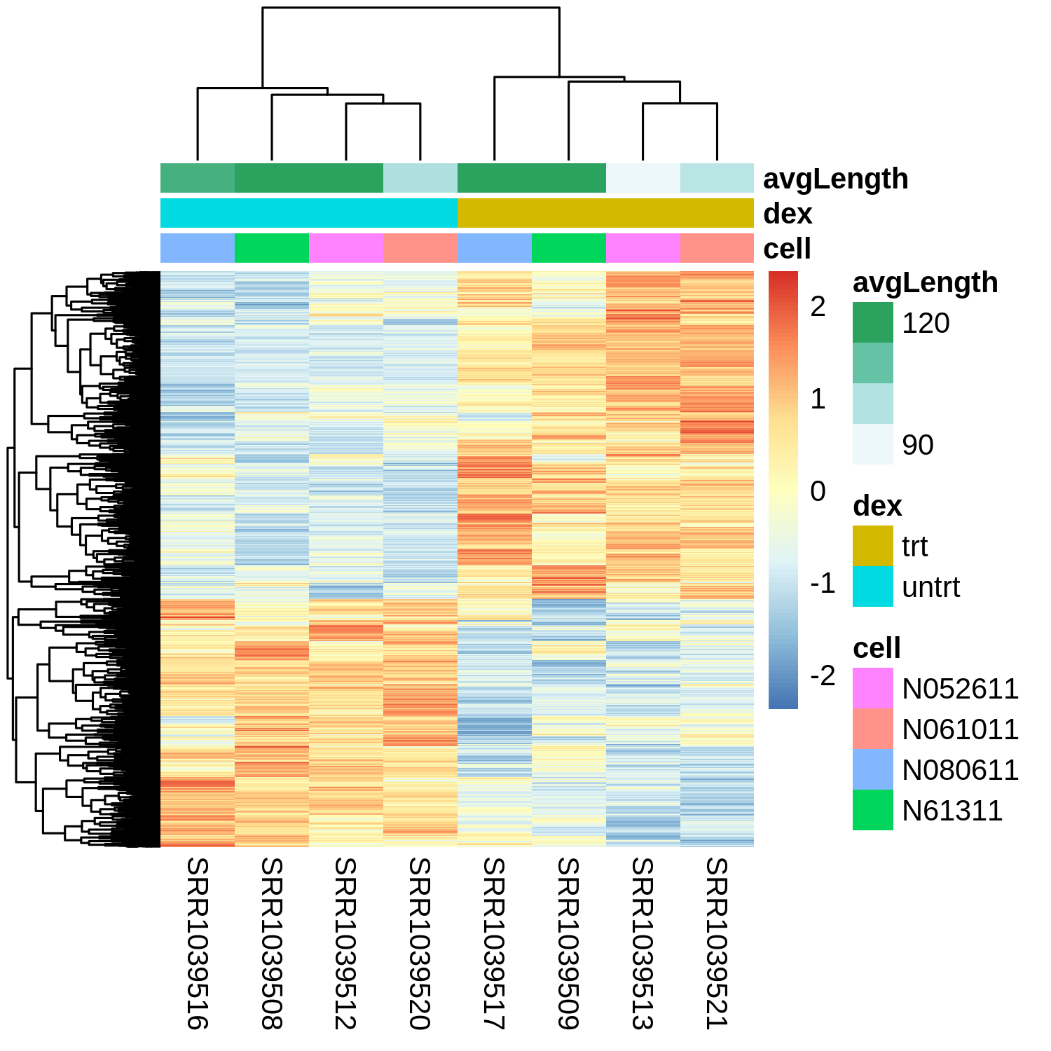
Looks like the samples separate primarily by treatment, as we would expect here since these are the differentially expressed genes.

We also see some variability by cell line, as we would have expected from the PCA plot.

Finally, we see a mix of genes upregulated vs. downregulated in the treated condition.

Visualizing differential expression statistics (scatterplots)

MA plot

In the above section, we only looked at the differentially expressed genes.

However, we may also want to look at patterns in the differential expression results overall, including genes that did not reach significance.

One common summary plot from differential expression is the MA plot.

In this plot, mean expression across samples (baseMean) is compared to log-fold-change, with genes colored by whether or not they meet the significance level we set for adjusted p-value (padj).

Generally for lowly expressed genes, the difference between conditions has to be stronger to create statistically significant results compared to highly expressed genes. The MA plot shows this effect.

DESeq2 has a nice function plotMA that will do this for you (using the output of the results function), and format everything nicely.

Add argument alpha=0.01 to set the adjusted p-value cutoff to 0.01 instead of the default 0.1.

plotMA(object = res,alpha=0.01)

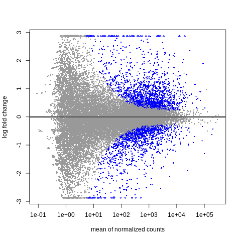
The x-axis here is log10-scaled. The y-axis here is log2(treated/untreated).

The blue dots are for significantly differentially expressed genes (padj < .01).

We find that at low baseMean (closer to 1e+01 or ~10), the magnitude of the log2-fold-change must be very large (often +/-2 or +/- 3, so something like 4-fold or 8-fold difference) for the gene to be significant.

Meanwhile at higher baseMean (say, as we go to 1e+03 or ~1000 reads and above), we find that the magnitude of the log2-fold-change can be much smaller (going down to +/- 0.5, so something like a 1.4-fold difference, or even less).

Volcano plot

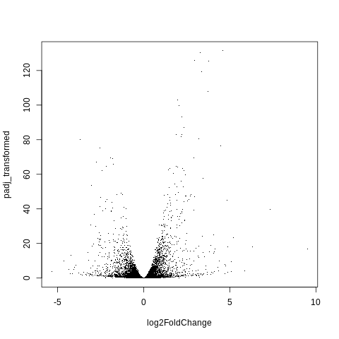
Another interesting plot is a volcano plot. This is a plot showing the relationship between the log2-fold-change and the adjusted p-value.

First, extract these two values from res.

Let’s refresh ourselves on what the column names are here.

colnames(res)

[1] "baseMean"       "log2FoldChange" "lfcSE"          "stat"          
[5] "pvalue"         "padj"

Extract columns log2FoldChange and padj into objects of the same name.

Solution

log2FoldChange = res$log2FoldChange
padj = res$padj

Plot log2FoldChange on the x-axis and padj on the y-axis.

Solution

plot(log2FoldChange,padj)

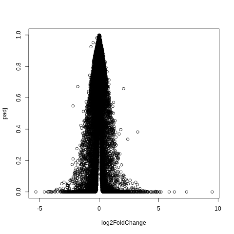
Add argument to make the points smaller.

Argument:

pch="."

Solution

plot(log2FoldChange,padj,pch=".")

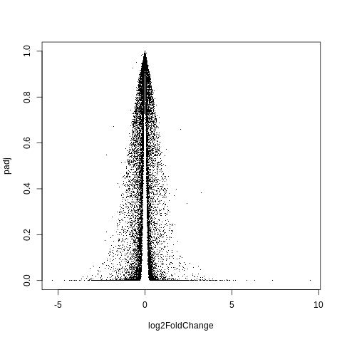
Hm, this still doesn’t look quite right.

If I search for what a volcano plot should look like, I get something closer to this.

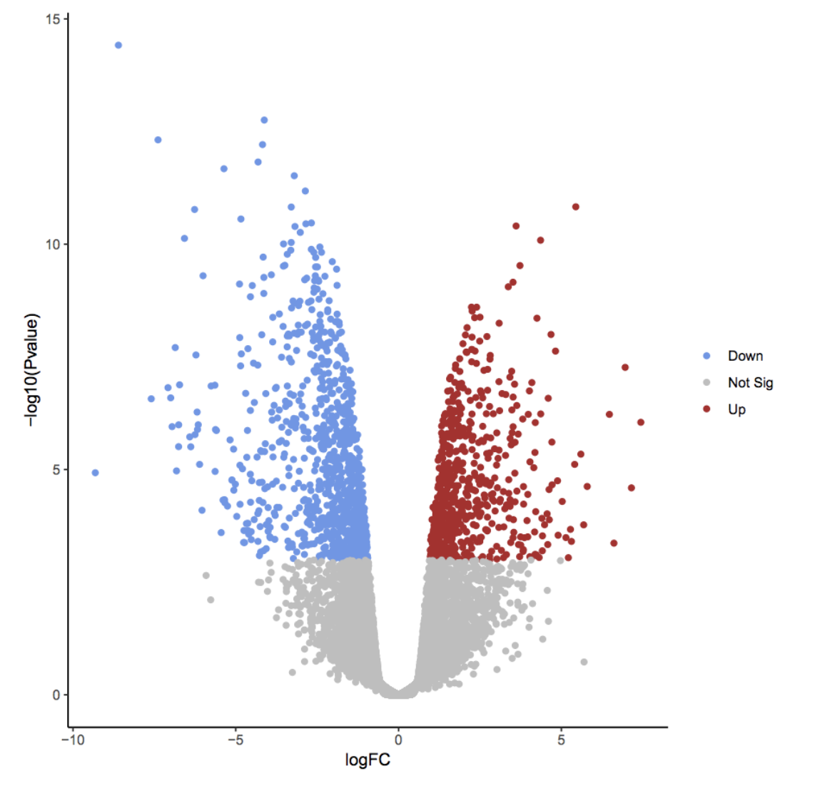
I believe we need to take -log10 of padj.

Let’s do that, and save as padj_transformed.

Then, redo plot using this new variable.

Solution

padj_transformed = -log10(padj)

plot(log2FoldChange,padj_transformed,pch=".")

Preparing files for functional enrichment (ORA/GSEA)

Next, we will want to take the results of differential expression testing, and prepare for input into functional enrichment, either over-representation (ORA) or gene set enrichment (GSEA) analysis.

Then, we will import these inputs to a web-based tool called WebGestalt.

In over-representation analysis, the idea is to test whether genes that are significantly differential expressed are enriched for certain categories of genes (gene sets). The input to this is a list of the gene IDs/names for the differentially expressed genes.

In gene set enrichment analysis, genes are ranked by how differential expressed they are, and whether they are upregulated or downregulated. The input to this is a table with the gene IDs/names of all genes, and the test-statistic (here the stat column), ordered by the test-statistic.

Preparing for input into ORA

Here, we will prepare the input for ORA by first getting all the gene IDs into an object called geneids.

These gene IDs are stored in the row names of the results (res), so we can get them out using the rownames function.

Solution

geneids = rownames(res)

Next, subset geneids to just the differentially expressed genes using the previously calculated indices (that we made for the heatmap step).

Syntax to subset an object using previously calculated indices.

x_subset = x[previously_calculated_indices]

Let’s output to an object called geneids.sig.

Solution

geneids.sig = geneids[degs]

Output to a text file called geneids_sig.txt using the writeLines command.

Let’s get the syntax for this command.

?writeLines

Usage:

     writeLines(text, con = stdout(), sep = "\n", useBytes = FALSE)
     
Arguments:

    text: A character vector

     con: A connection object or a character string.

There is no example in the help message, but I found one on Stack Overflow that may be helpful (paraphrased below).

mywords = c("Hello","World")
output_file = "output.txt"
writeLines(text = mywords, con = output_file)

Let’s run this here.

Solution

output_file = geneids_sig.txt

writeLines(text = geneids.sig, con = output_file)

Error: object 'geneids_sig.txt' not found

Oops, let’s fix.

Solution

output_file = "geneids_sig.txt"

writeLines(text = geneids.sig, con = output_file)

Go to the Terminal tab, and let’s look at this file in more detail.

First, do head and tail.

head geneids_sig.txt

ENSG00000000003
ENSG00000000971
ENSG00000001167
ENSG00000002834
ENSG00000003096
ENSG00000003402
ENSG00000004059
ENSG00000004487
ENSG00000004700
ENSG00000004799

tail geneids_sig.txt

ENSG00000272695
ENSG00000272761
ENSG00000272796
ENSG00000272841
ENSG00000272870
ENSG00000273038
ENSG00000273131
ENSG00000273179
ENSG00000273259
ENSG00000273290

Also check number of lines.

wc -l geneids_sig.txt

2901 geneids_sig.txt

All looks good.

Normally, you would download the file you just created to your laptop, but we may not always have a way to transfer files from the cloud VM to your laptop. So, let’s download the file from the Github for this workshop. Download link here.

Preparing for input into GSEA

Let’s move on to creating the input for GSEA. This will be a data frame with two columns.

• gene : The gene ID (already have these for all genes in geneids)
• stat : The stat column from the differential expression results (res)

We will use the data.frame function here.

?data.frame

Examples:

L3 <- LETTERS[1:3]
char <- sample(L3, 10, replace = TRUE)
d <- data.frame(x = 1, y = 1:10, char = char)

Let’s call this data frame gsea.input.

Solution

gsea.input = data.frame(gene = geneids,
    stat = res$stat)

Sort by the stat column.

Solution

order_genes = order(gsea.input$stat)

gsea.input = gsea.input[order_genes,]

Output to a tab-delimited text file gsea_input.txt using the write.table function.

Solution

output_file = "gsea_input.txt"
write.table(x = gsea.input,file=output_file,sep="\t")

Let’s switch over to the Terminal tab and look at this file in more detail.

head gsea_input.txt

"gene"	"stat"
"10923"	"ENSG00000162692"	-19.4160587914648
"14737"	"ENSG00000178695"	-18.8066074036207
"3453"	"ENSG00000107562"	-18.0775817519565
"9240"	"ENSG00000148848"	-18.0580936880167
"8911"	"ENSG00000146250"	-17.7950173361052
"3402"	"ENSG00000106976"	-17.6137734750388
"11121"	"ENSG00000163394"	-17.4484303669187
"5627"	"ENSG00000124766"	-17.1299063626842
"3259"	"ENSG00000105989"	-15.8949963870475

Info on formatting of the file for input into GSEA available here, from the Broad Institute’s documentation.

This says that there should be two columns - one for the feature identifiers (i.e. gene IDs or symbols) and one for the weight of the gene (here, the stat column). But our output has three columns - this is not what we want.

Let’s go back to the R notebook tab and see if we can fix this.

Comparing to the example in the file format documentation, it seems we should do the following:

• Remove the quotation marks.
• Remove the header.
• Remove the first column.

Go back to R and see if we can find arguments in the read.table function to help with this.

?read.table

Arguments:

quote: a logical value (‘TRUE’ or ‘FALSE’) or a numeric vector.  If
          ‘TRUE’, any character or factor columns will be surrounded by
          double quotes.  If a numeric vector, its elements are taken
          as the indices of columns to quote.  In both cases, row and
          column names are quoted if they are written.  If ‘FALSE’,
          nothing is quoted.
row.names: either a logical value indicating whether the row names of
          ‘x’ are to be written along with ‘x’, or a character vector
          of row names to be written.

col.names: either a logical value indicating whether the column names
          of ‘x’ are to be written along with ‘x’, or a character
          vector of column names to be written.  See the section on
          ‘CSV files’ for the meaning of ‘col.names = NA’.

Looks like we need to add a few arguments to get our output formatted correctly.

Let’s output to a new file gsea_input_corrected.txt.

Solution

output_file = "gsea_input_corrected.txt"
write.table(x = gsea.input,file=output_file,sep="\t",row.names=FALSE,col.names=FALSE,quote=FALSE)

Go back to the Terminal tab, and look at this file again.

head gsea_input_corrected.txt

ENSG00000162692	-19.4160587914648
ENSG00000178695	-18.8066074036207
ENSG00000107562	-18.0775817519565
ENSG00000148848	-18.0580936880167
ENSG00000146250	-17.7950173361052
ENSG00000106976	-17.6137734750388
ENSG00000163394	-17.4484303669187
ENSG00000124766	-17.1299063626842
ENSG00000105989	-15.8949963870475
ENSG00000108821	-15.2668170602372

Looks ok - what about tail?

tail gsea_input_corrected.txt

ENSG00000273470	NA
ENSG00000273471	NA
ENSG00000273475	NA
ENSG00000273479	NA
ENSG00000273480	NA
ENSG00000273481	NA
ENSG00000273482	NA
ENSG00000273484	NA
ENSG00000273490	NA
ENSG00000273491	NA

Let’s also check the line count.

wc -l gsea_input_corrected.txt

63677 gsea_input_corrected.txt

Hm - don’t think we should be including genes with an NA for the stat column?

Let’s fix again.

Let’s use grep to remove lines with “NA”, and output to a new file gsea_input_corrected_minus_NA.txt.

Solution

grep -v NA gsea_input_corrected.txt > gsea_input_corrected_minus_NA.txt

Check again.

head gsea_input_corrected_minus_NA.txt

ENSG00000162692	-19.4160587914648
ENSG00000178695	-18.8066074036207
ENSG00000107562	-18.0775817519565
ENSG00000148848	-18.0580936880167
ENSG00000146250	-17.7950173361052
ENSG00000106976	-17.6137734750388
ENSG00000163394	-17.4484303669187
ENSG00000124766	-17.1299063626842
ENSG00000105989	-15.8949963870475
ENSG00000108821	-15.2668170602372

tail gsea_input_corrected_minus_NA.txt

ENSG00000154734	20.2542354089516
ENSG00000125148	20.9292144890544
ENSG00000162614	21.6140905458227
ENSG00000157214	21.968453609644
ENSG00000211445	22.4952633774851
ENSG00000189221	23.6530144138538
ENSG00000101347	24.2347153246759
ENSG00000120129	24.2742584224751
ENSG00000165995	24.7125510867281
ENSG00000152583	24.8561114516005

wc -l gsea_input_corrected_minus_NA.txt

33469 gsea_input_corrected_minus_NA.txt

We now have fewer lines, because we removed the lines for the genes with an “NA” in the stat column.

You can download a copy of this file here.

Running functional enrichment (ORA/GSEA)

Let’s head to the website WebGestalt.

Run ORA

Click “Click to upload” next to “Upload ID List”.

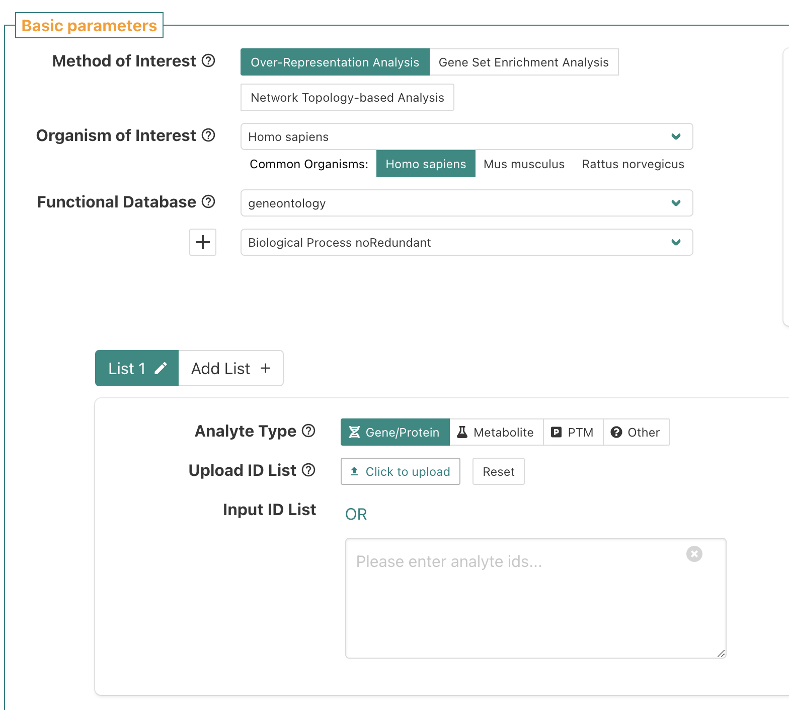
Upload geneids_sig.txt.

For the reference set, select “genome protein-coding”.

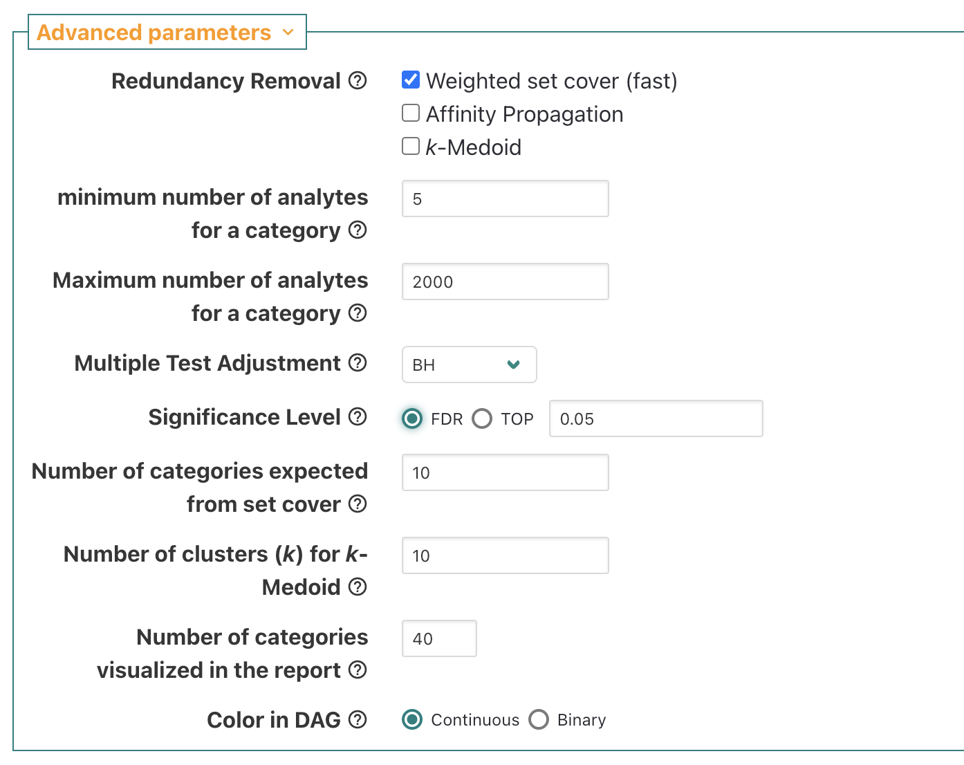
In advanced parameters, switch from top 10 to FDR 0.05.

Let’s look at the results!

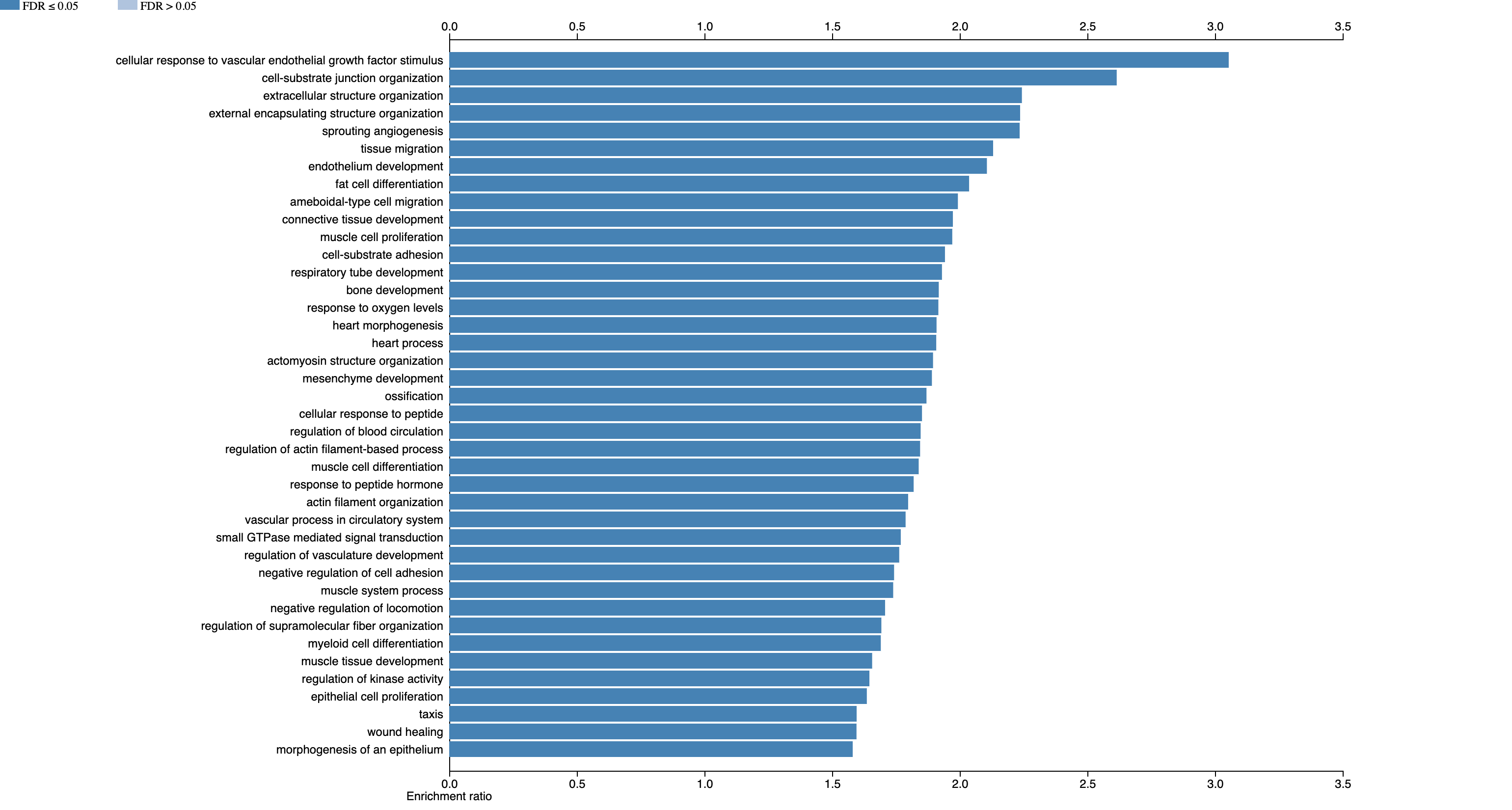
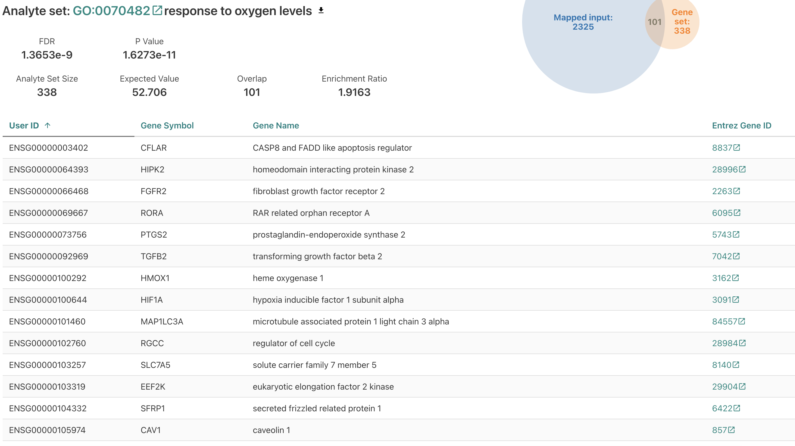
Let’s scroll down and click on “response to oxygen levels”, as this seems pretty relevant for an airway dataset.

We can scroll through and look at the genes that are in this gene set, that are differentially expressed.

Run GSEA.

Let’s move on to running gene set enrichment analysis (GSEA).

For the tab at the top, switch to “Gene Set Enrichment Analysis”.

Switch back the functional database to the same as before (geneontology, Biological Process noRedundant).

This time, upload gsea_input_corrected_minus_NA.txt.

Also reset the advanced parameters to select based on FDR of 0.05 rather than the top 10 again.

We get the following error message.

Turns out, this is as simple as renaming the file!

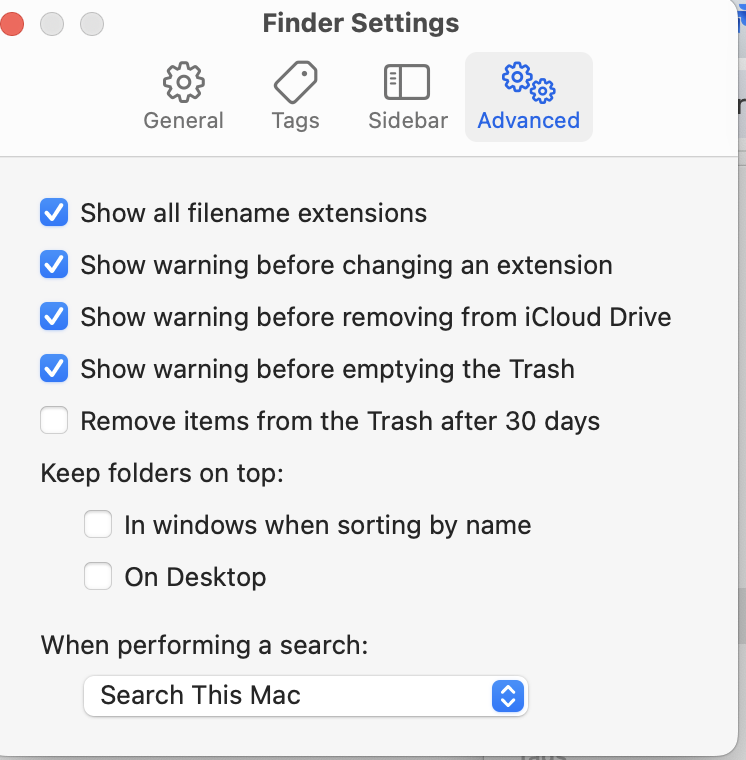
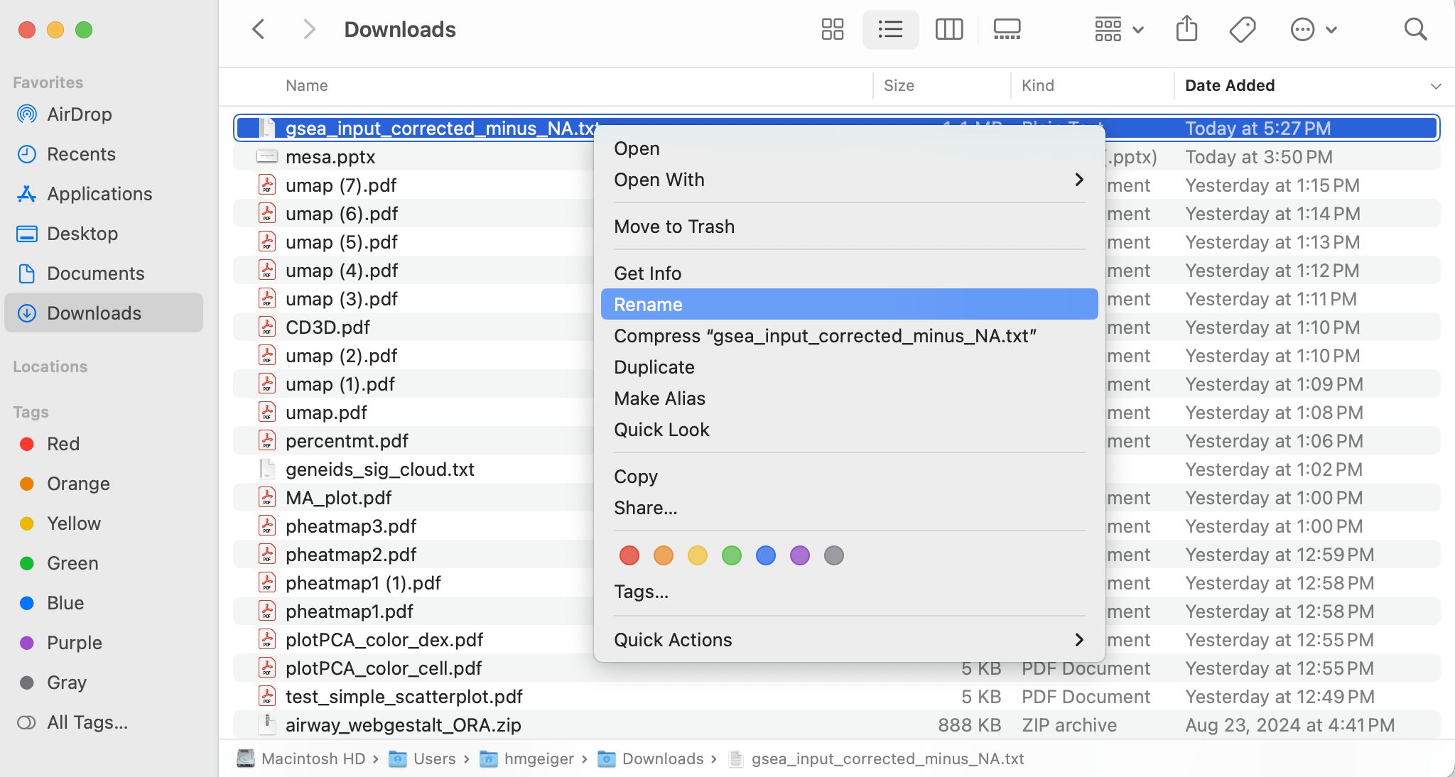
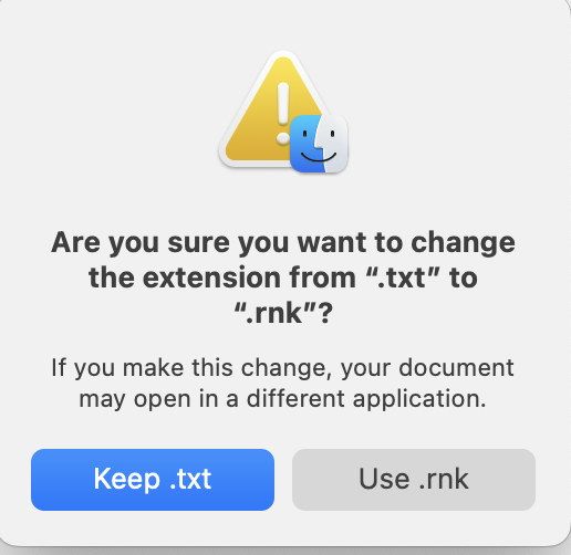
Let’s change the file suffix to “.rnk” instead of “.txt” (rename the file).

Below is shown how to do this using Mac’s Finder program - you can do this however you would normally for your system.

Now, go back and redo all of the above, but input gsea_input_corrected_minus_NA.rnk.

This time it should work, and output something like the following:

Hm - fewer categories than we might have expected?

Let’s redo, but change functional database to pathway = Kegg.

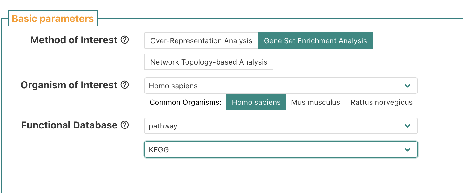
Click on autophagy.

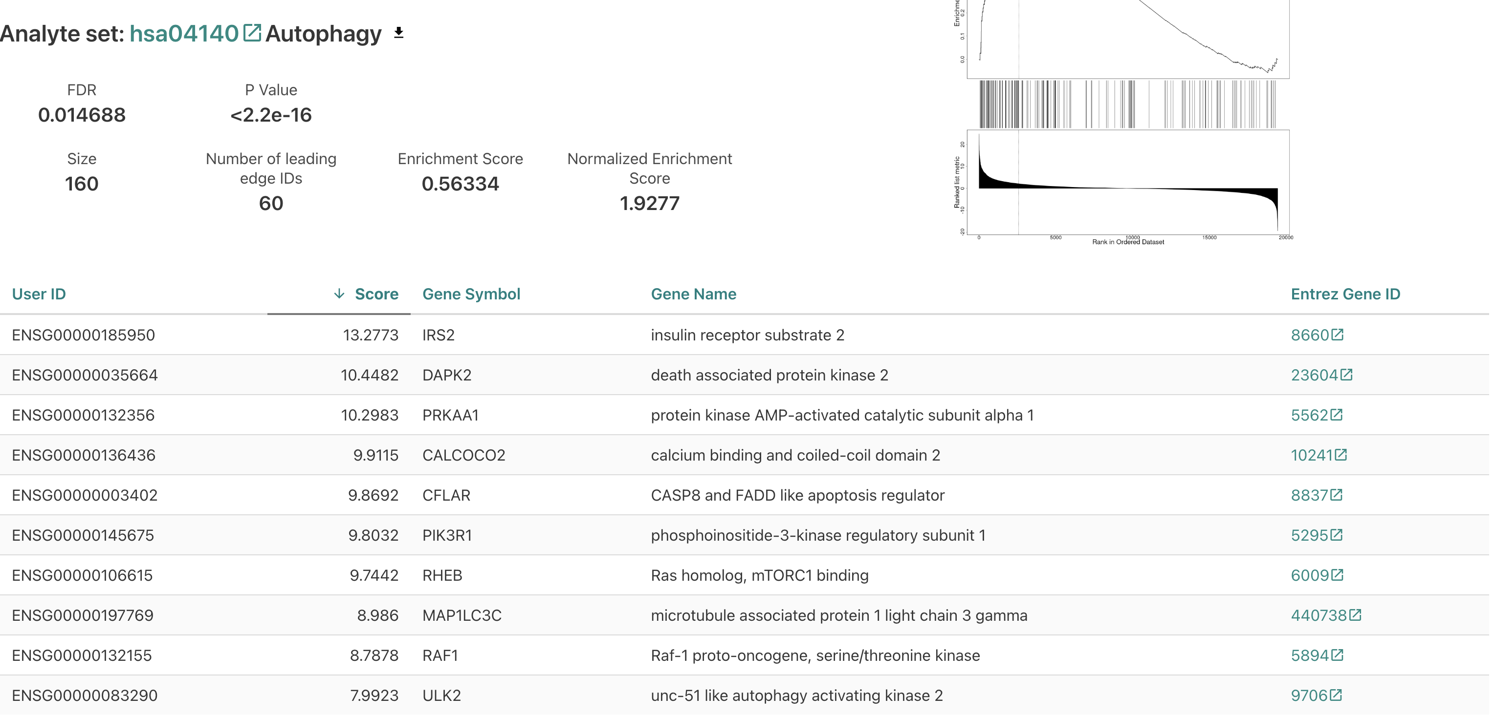
Nice! For this test we also get a value that gives the relative magnitude of change (here, all the categories seem to be ones associated with genes upregulated upon treatment).

Key Points

• Normalization is necessary to account for different library sizes between samples.

• Dimensional reduction (PCA) can help us understand the relationship between samples, and how it tracks with biological and technical variables.

• We often want to include technical variables in the design formula, so that the differential expression comparison may include controlling for these as we solve for the effect of the biological variable.

• Heatmaps are a useful visualization for understanding differential expression results, but must often be scaled by gene to become interpretable.

• ORA and GSEA accept very different inputs (only DE genes versus all genes), and their outputs may be different as well as a result (though often they include similar categories).